Simulating Convergence

TL;DR

Theme: Convergence helps answer the limiting behaviour of a sequence of random variables.

Types of Convergence:

• Convergence in probability.

• Convergence in distribution.

• Convergence in quadratic mean.

Main results:

• Law of Large Numbers - Given a sequence of i.i.d random variables, Mean of a large sample is close to the mean of it’s distribution.

• Central Limit Theorem - Given a sequence of i.i.d random variables with some mean and variance, distribution of an operation on this sequence (i.e mean/sum/sqrt of sum etc.) tends to a normal distribution as the number of the random variables increase.

Convergence in probability

Def-1: Let \(X_1, X_2, ...\) be a sequence of random variables and let \(X\) be another random variable. Then, \(X_n\) converges to \(X\) in probability, i.e

\[X_n \xrightarrow{P} X, \\ \text{if for every} \ \epsilon > 0, \\ P(|X_n - X| > \epsilon) \rightarrow 0 \\ \text{as} \ n \rightarrow \infty\]

This phenomenon is particularly useful while inferencing population parameters from a sample.

This concept can be used to build up WLLN which is stated as:

Theorem - 1, Weak Law of Large Numbers (WLLN): \(\text{If} \ X_1,X_2,...,X_n \ \text{are i.i.d then} \ \bar{X_n} \xrightarrow{P} \mu\)

This means that as the sample size increases, the sample mean gets centered around the population mean.

Let’s build deeper intuition of WLLN using a simple example.

Example-1: Say \(X\) is a R.V that is normally distributed with population mean, \(\mu = 5\). Now, as per WLLN as the sample size increases sample mean, \(\bar{X}\), should get closer to 5.

import numpy as np
import random
import matplotlib
import matplotlib.pyplot as plt
import tensorflow as tf
import tensorflow_probability as tfp#Setting some global plot parameters
matplotlib.rc('xtick', color = 'white')
matplotlib.rc('ytick', color = 'white')
matplotlib.rc('axes', edgecolor = 'white')
matplotlib.rc('text', color = 'white')
matplotlib.rc('axes', labelcolor = 'white')

try:
  tf.compat.v1.enable_eager_execution()
except ValueError:
  pass

tfd = tfp.distributions

#Create a normal distribution with mean = 5 and pull one sample at a time
ex1_dist = tfd.Normal(loc = 5, scale = 1)
ex1_rvs = np.zeros(20000)
for i in range(20000): #Pull one sample at a time
  ex1_rvs[i] = ex1_dist.sample(1)

#Compute sample mean for increasing sample sizes at an interval of 100
sample_mean = lambda sample: np.mean(sample)
iter_array = np.arange(0,20000,100)
sample_mean_list = []
for i in iter_array:
  sample_mean_list.append(sample_mean(ex1_rvs[:i]))
#Plot sample mean for increasing sample sizes
plt.figure(figsize=(10,6))
plt.plot(iter_array, sample_mean_list, color = 'royalblue')
plt.yticks(np.arange(4.8,5.2,0.05))
plt.axhline(y=5, color='r', linestyle='--')
plt.title("Weak Law of Large Numbers (WLLN), in action")
plt.xlabel("Sample Size")
plt.ylabel("Sample Mean")
plt.show()

/usr/local/lib/python3.6/dist-packages/numpy/core/fromnumeric.py:3335: RuntimeWarning: Mean of empty slice.
  out=out, **kwargs)
/usr/local/lib/python3.6/dist-packages/numpy/core/_methods.py:161: RuntimeWarning: invalid value encountered in double_scalars
  ret = ret.dtype.type(ret / rcount)

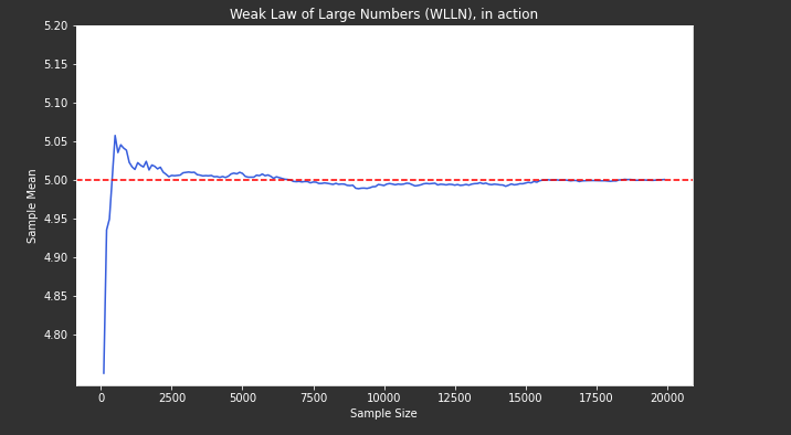
• We can observe that as the sample size increases, sample mean gets centered around the population mean, \(\mu = 5\).

Convergence in Distribution

Def-2: Let \(X_1, X_2, ...\) be a sequence of random variables and let \(X\) be another random variable. Let \(F_n\) denote the CDF of \(X_n\) and let \(F\) denote the CDF of X. Then, \(X_n\) converges to \(X\) in distribution i.e \(X_n \xrightarrow{D} X\) if,

\[lim_{n \rightarrow \infty} F_n(t) = F(t)\]

at all \(t\) for which F is continuous.

This notion helps build up CLT (Central Limit Theorem) which says that sum of a large number of independent random variables each with a finite mean and variance has a distribution that is approximately normal. A simple formalization is as follows:

Theorem-2, The central limit theorem: Let X_1, X_2,… be a sequence of i.i.d random variable, each with mean \(\mu\) and variance \(\sigma^2\). Let \(S_n = \sum_{i=1}^n X_i\) Then the distribution of

\(\frac{S_n-n \mu}{\sigma \sqrt n} \xrightarrow{D} Z\) where \(Z\) is the standard normal, \(Z ~ N(0,1)\), as \(n \rightarrow \infty\).

Let us emperically observe a few examples of CLT:

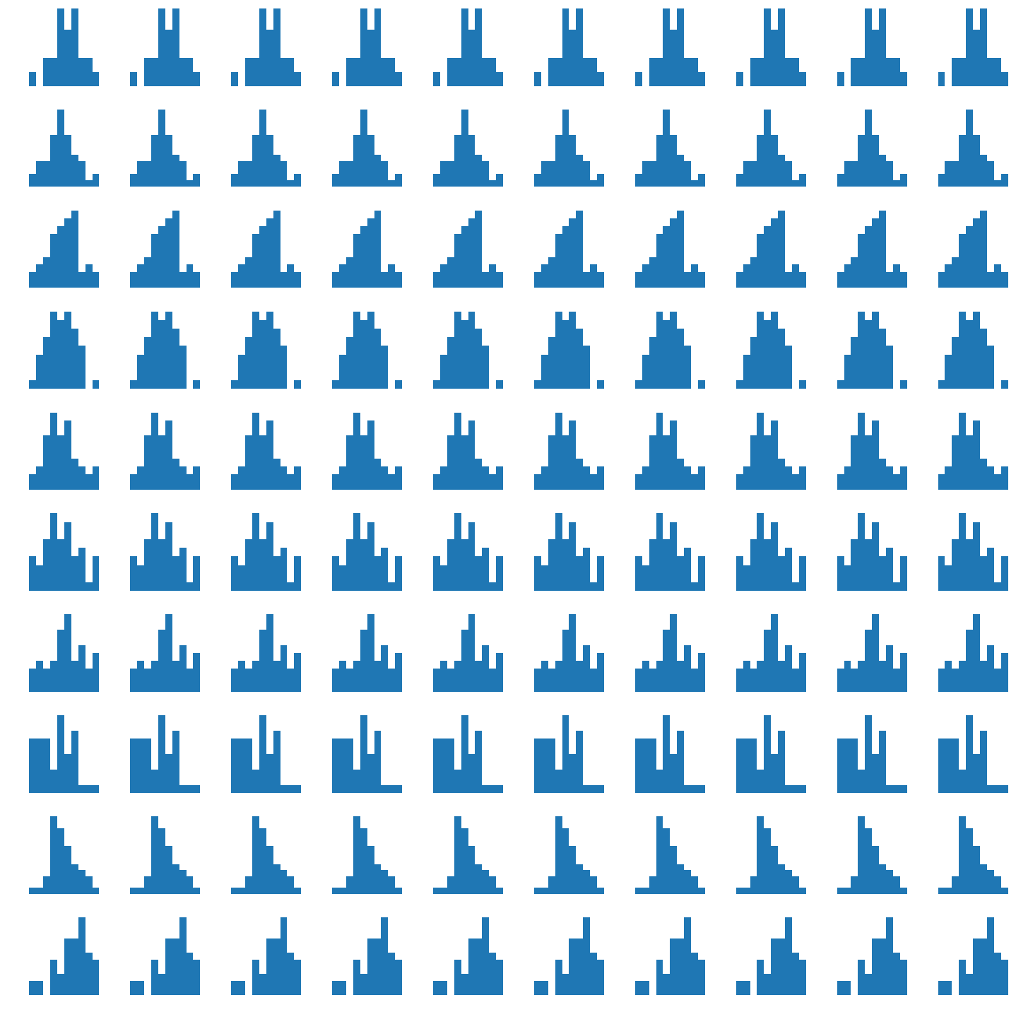
#First let's generate 500 i.i.d random variables
mean = 5
var = np.arange(0.5, 2, 0.5)
rv_sequence = []
i = 0
while i <= 1000:
  v = float(random.choices(var)[0])
  ex2_dist = tfd.Normal(loc = mean, scale = v)
  rv_sequence.append(ex2_dist.sample(50))
  i += 1

#Plot histograms for every 5th sample
fig, ax = plt.subplots(nrows = 10, ncols = 10, figsize=(20, 20))
for i in range(10):
  for j in range(10):
    ax[i][j].hist(rv_sequence[i*5])
fig.tight_layout()

#Get mean of each sample
rv_sequence_mean = [np.mean(i) for i in rv_sequence]
#Plot distribution of sample means
plt.hist(rv_sequence_mean)
plt.axvline(x=5, color='r', linestyle='--')
plt.title("Distribution of sample means")
plt.xlabel("Sample Means")
plt.show()

#Get sum of each sample
rv_sequence_sum = [np.sum(i) for i in rv_sequence]
#Plot distribution of sample means
plt.hist(rv_sequence_sum)
plt.axvline(x=250, color='r', linestyle='--')
plt.title("Distribution of sample sums")
plt.xlabel("Sample Sums")
plt.show()

#Get max of each sample
rv_sequence_sum_sqrt = [np.sqrt(np.sum((i))) for i in rv_sequence]
#Plot distribution of sample max
plt.hist(rv_sequence_sum_sqrt)
plt.axvline(x=15.75, color='r', linestyle='--')
plt.title("Distribution of sqrt of sample sum")
plt.xlabel("Sample Sum Sqrt")
plt.show()

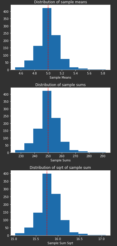
• Observe how that the distribution of sample means takes the shape of a gaussian with it’s location at the population mean value of 5.
• Observe how that the distribution of sample sum/sqrt. of sample sum has a normal distribution with a certain mean.