All Things Markov
Stochastic process
Stochastic process is a system that evolves randomly in time. This system can be charecterized by a collection of random variables, \(\{X(\tau), \tau \in T\}\) where \(T\) is the parameter set. The values these random variables can take is given by the state space, \(S\). If the system is discrete it can be represented as \(\{X_n, n \geq 0\}\) (intuitively this means we observe the system in discrete points in time). If continous \(\{X(t), t \geq 0\}\), here we observe the system continuously.
In the above definition, we are saying that the input to this Stochastic process is in the parameter set \((T)\) and the output is in the state space \((S)\). That means, a stochastic process has to be some type of a function that maps values from parameter space to state space? As it turns out, stochastic process is a special type of a function.
Formally, we can define \(x: T \rightarrow S\) then we can consider \(\{x(\tau), \tau \in T\}\) to be an evolution trajectory of \(\{X(\tau), \tau \in T\}\). These functions \(x\) are called sample paths of the stochastic process. Naturally, there could uncountable sample paths. Since our stochastic process follows one of the sample paths randomly, it is called a random function. If we are able to understand the behaviour of these random sample paths then we can predict the outcome of our system.
Many times it’s useful to convert a continous time stochastic process into a discrete time one by assuming that we observe the system in discrete points in time.
How do we charecterize a stochastic process?
We mentioned above that a stochastic process is a collection of random variable. Therefore, abstractly speaking there exists a probability space, \((\Omega, \mathcal{F}, P)\), on which the process is defined.
Q1-1. Now the question is how do we represent/describe this probability space?
For the discrete case:
-
If \(T\) is finite, then we can represent the system using it’s joint CDF i.e \(F(x_1,x_2,x_3,...,x_n) = P(X_1 \leq x_1, X_2 \leq x_2, ..., X_n \leq x_n)\)
-
What if \(T\) is infinite? Then the above expression would be 0 or 1 for many cases. So what do we do? Turns out, in such cases we can represent it using a “consistent” family of finite dimensional joint CDFs \(\{F_n, n \geq 0\}\) \(F(x_1,x_2,x_3,...,x_n) = P(X_1 \leq x_1, X_2 \leq x_2, ..., X_n \leq x_n) \\ \forall -\infty \leq x_i \leq \infty \ and \ i = 0,1,2...,n\) where this family is called “consistent” if: \(F_n(x_1,x_2,...,x_n) = F_{n+1}(x_1,x_2,...,\infty) \\ \forall -\infty \leq x_i \leq \infty \ and \ i = 0,1,2...,n, n \geq 0.\)
Intuitively, this means that any probabilistic question about a discrete time stochastic process \(\{X_n, n \geq 0\}\) can be answered in terms of \(\{F_n, n\geq 0\}\).
Example: Let \(\{X_n, n \geq 1\}\) be a sequence of iid random variables completely described by distribution \(F(.)\) as we can create a consistent family of joint CDFs such as \(F_n(x_1,x_2,...,x_n) = \prod_{i=1}^n F(x_i)\). Now let \(S_0 = 0\), \(S_n = \sum_{i=1}^n X_i\), \(n \geq 1\). This \(\{S_n, n \geq 0\}\) is called a random walk which is completely charecterize by \(F(.)\) since \((S_i)_{i=1}^n\) are completely determined by \((X_i)_{i=1}^n\).
Discrete Time Markov Chain
Definitions
Def 1, Markov Property: “If the present state of the system is known, the future of the system is independent of it’s past.”
One interpretation: Past affects the future of a system only via the present.
Another interpretation: Present state of the system contains all the information to predict the future state of the system.
Def 2, Discrete Time Markov Chain (DTMC): Stochastic process \(\{X_n, n \geq 0\}\) with countable state space \(S\) is a DTMC if: \(P(X_{n+1} = j | X_n = i, X_{n-1}, X_{n-2}, ..., X_0) = P(X_{n+1} = j | X_{n} = i) \\ \forall n \geq 0, X_n \in S \\ \forall n \geq 0, i,j \in S\)
Informally: Stochastic process \(\{X_n, n \geq 0\}\) with countable state space \(S\) adhering to the Markov Property is a DTMC.
Def 3, Time-Homogeneity: DTMC \(\{X_n, n \geq 0\}\) with countable state space \(S\) is said to be time-homogeneous if: \(P(X_{n+1} = j | X_{n} = i) = p_{i,j} \forall n \geq 0, i,j \in S\)
This \(p_{i,j}\) is called the transition probability from state \(i\) to \(j\).
Matrix housing \(p_{i,j} \forall i,j\) is called one-step transition probability matrix. When \(S\) is finite with a total of \(m\) values, this matrix can be represented as a \(m*m\) square matrix. Note that, this one step transition probability matrix is a stochastic matrix (i.e row’s sum upto 1 and each value is \(\geq 0\)).
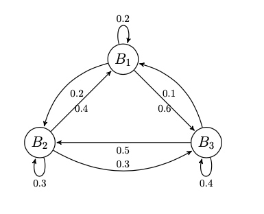
Running Example: Imagine we have a friend - \(\pi\) who is a fitness enthusiast and chooses among three brands of vegan protein - \(B_1, B_2, B_3\) every month when he makes a purchase. We have been tracking his purchase behaviour and have modelled it as a DTMC \(\{X_n, n \geq 0\}\) with state space \(S = \{B_1, B_2, B_3\}\), and a transition probability matrix \(P\) as follows: \(\begin{bmatrix} 0.2 & 0.2 & 0.6\\ 0.4 & 0.3 & 0.3\\ 0.1 & 0.5 & 0.4\\ \end{bmatrix}\)
\(\pi\) has a sibling \(\veebar\) who is about to get into fitness and we assume his taste would mimic \(\pi\). However, since \(\veebar\) has no idea which one to choose first (as he doesn’t want to ask \(\pi\)) his decision is influenced by these brands marketing efforts. Let’s assume his nudge is captured by the initial distribution vector [0.5,0.3,0.2].
We can also represent this transition probability matrix as a Graph - called transition diagram where nodes of this graph is equal to the state space. Here is the transition probability matrix from our example as a graph:
ex_tpm = np.array([0.2,0.2,0.6,0.4,0.3,0.3,0.1,0.5,0.4]).reshape(3,3)
ex_inidist = np.array([0.5,0.3,0.2]).reshape(1,3)
Charecterization of a DTMC
In order to charecterize a DTMC we need to represent/describe the distribution of it’s elements i.e \((X)_i's\).
Q2-1. How do we that?
Intuitively: We currently have the transition probability matrix mentioned above but it only has information related to conditional probabilities. Due to Markov Property and Time Homogeneity, we can use it to completely describe our DTMC provided our system is in process (\(X_1\) and beyond) but it doesn’t tell us how our system was at the very begining. Therefore, we need to add more information about our system’s initial behaviour. This can be done by specifying the distribution of \(X_0\) externally (Since \(X_0\) is a discrete R.V, we can use the PMF): \(a_i = P(X_0 = i), i \in S \\ \textbf{a} = [a_i]_{i \in S}\) Therefore, \(\textbf{a}\) is the PMF of \(X_0\) and since it is the PMF of \(X_0\), which is the initial state of our DTMC, we call it the initial distribution of the DTMC.
Now we know: 1) The initial distribution of our DTMC. (Specified as PMF of \(X_0\)) 2) How it changes at any step \(X_{n+1}\) is given only by step \(X_n\) (Markov Property) and it is captured by \(p_{i,j}\) (Time Homogeneity). 3) Since, change begins at \(X_0\) whose distribution we are specifying and thereafter have probabilities assosiated with corresponding changes we have the entire chain figured out.
Formally: Theorem 1, Charecterization of a DTMC. A DTMC is completely determined by it’s initial distribution and it’s probability transition matrix.
We can prove it by showing that we can compute the finite dimensional joint probability mass function \(P(X_0 = i_0, X_i = i_1, ..., X_n = i_n)\) where \(i \in S\) in terms of \(a\) and \(P\). \(P(X_0 = i_0, X_i = i_1, ..., X_n = i_n) = \\ P(X_n = i_n | X_{n-1} = i_{n-1}, ..., X_i = i_1, X_0 = i_0) * P(X_{n-1} = i_{n-1}, ..., X_i = i_1, X_0 = i_0) \\ P(X_n = i_n | X_{n-1} = i_{n-1}) * P(X_{n-1} = i_{n-1}, ..., X_i = i_1, X_0 = i_0) - \text{Markov Property} \\ p_{i_{n-1}, i_n} * P(X_{n-1} = i_{n-1}, ..., X_i = i_1, X_0 = i_0) - \text{Time Homogeneity} \\ p_{i_{n-1}, i_n}p_{i_{n-2}, i_{n-1}}...p_{i_{0}, i_{1}}a_{i_0} - \text{Induction}\)
Transient Behaviour
Marginal Distribution
Q3-1. What are some obvious things that would be useful for us to learn about this DTMC?
Something that would be particularly useful would be to obtain the distribution of our DTMC at a given interval. This will help us probabilistically answer what value our system will take on a given day (assuming we are measuring our system daily). We can do this by computing the PMF of \(X_n\).
Q3-2. How do we find it?
Intuitively: The easiest way to figure this out is to understand how our system behaves at the start (which is something we already have - initial distribution, denoted by \(\mathbf{a}\)) and then charecterize how our system has changed up until that moment i.e up until \(X_n\). The obvious next question would be, how do we charecterize this change quantitatively? One way to do that would be to compute \(P(X_n = j | X_0 = i), i,j \in S\), i.e compute the n-step transition probability.
Formally: To find the marginal distribution of \(X_n\) we can sum it over all R.V’s, \(X_{n-1},X_{n-2},...,X_0\), up until that point. But this is tedious instead since we know \(X_0\) if we can find out \(P(X_n = j | X_0 = i), i,j \in S\) our task is greatly simplified. Using the idea of marginalization over \(X_0, \\ P(X_n = j) = \sum_{i \in S} P(X_n = j, X_0 = i)\\ = \sum_{i \in S} P(X_n = j | X_0 = i) P(X_0 = i) \\ = \sum_{i \in S}p^n_{i,j}a_i \ where \ i,j \in S, n \geq 0\)
where \(p^n_{i,j}\) is the n-step transition probability i.e the probability of going from state \(i\) to state \(j\) in \(n\) steps.
Q3-3. How do we compute \(p^n_{i,j}\)?
Intuitively: If \(X_n\) is \(X_1\) i.e \(n=1\) then it is pretty straight forward. However, when that is not the case we can think of going from \(i\) to \(j\) as going to an intermediate state \(r\) at a time \(k \leq n\) and then going from our intermediate state \(r\) to \(j\) in the remaining \(n-k\) steps.
Formally: Theorem 2, Chapman–Kolmogorov Equations. The n-step transition probabilities satisfy the following equations \(p^{(n)}_{i,j} = P(X_n = j | X_0 = i) \\ = \sum_r = p^{(k)}_{i,r}p^{(n-k)}_{r,j}\) where k is a fixed integer such that \(0 \leq k \leq n\).
Proving this is pretty straightforward, post that intuition: \(p^{(n)}_{i,j} = P(X_n = j | X_0 = i) \\ = \sum_{r \in S} P(X_n = j, X_k = r | X_0 = i) - \text{intermediate state} \\ = \sum_{r \in S} P(X_n = j | X_k = r, X_0 = i) P(X_k = r | X_0 = i) \\ = \sum_{r \in S} P(X_n = j | X_k = r) P(X_k = r | X_0 = i) - \text{Markov Property} \\ = \sum_{r \in S} P(X_n = j | X_0 = r) P(X_k = r | X_0 = i) - \text{Time Homogeneity} \\ = \sum_{r \in S} p^{(n-k)}_{r,j} p^{(k)}_{i,r}\)
In matrix form, \(\mathbf{P}^{(n)} = \mathbf{P}^{(n-k)}\mathbf{P}^{(k)} \ where \ 0 \leq k \leq n\). \(\mathbf{P}^{(n)}\) is the n-step transition probability matrix.
Okay, so now we have the missing piece. Now we can formally define the PMF of \(X_n\).
Formally: Theorem 3, PMF of \(X_n\).
For notation convenience let \(P(X_n = j), j \in S\) be \(\mathbf{a}^{(n)}\). Then, \(\mathbf{a}^{(n)} = \mathbf{a}^{(0)}\mathbf{P}^{(n)}\)
Q3-4. Computationally, how do we perform this operation?
Turns out \(\mathbf{P}^{(n)}\) is simply \(\mathbf{P}\) to the power of \(n\) (Can be proved via induction). This can be easily computed using a linear algebra module.
Also note that, if we know the initial state of our system i.e \(X_0 = i\) then the i-th row of \(\mathbf{P}^{n}\) gives the conditional pmf of \(X_n\).
For our running example, say it is \(\veebar\)’s birthday in 2 months and we want to buy him one of the 3 protein powders. Understanding the distribution of \(X_2\) can help us make a better purchase. This can be computed as follows:
dtmc = DTMC()
dtmc.pmf(ex_inidist, ex_tpm, 2)
dtmc.pmf_
This gives [0.211, 0.37 , 0.419]. This means although there was a greater chance that \(\veebar\) would buy \(B_1\) initially, his choice has changed and in regards to that it would make more sense for us to buy \(B_3\) for his birthday.
Occupancy Times
Suppose we have a finite state space where a few or all states are of primary importance, then understanding the amount of time spent in those states is particularly useful. This is what occupancy times helps us study.
Let \(V_j^{(n)}\) be the number of visits to state \(j\) by the DTMC with state space \(\{0,1,2,...,n\}\). This \(V_j^{(n)}\) is a R.V. Now, occupancy time i.e expected time spent by the DTMC in state \(j\) upto time \(n\) starting from state \(i\) is \(M_{i,j}^{(n)} = E(V_j^{(n)}|X_0 = i), i,j \in S, n \geq 0\).
Occupancy matrix is simply, \(\mathbf{M}^{(n)} = [M^{(n)}_{i,j}]\).
Q4-1. How do we compute occupancy time matrix (\(\mathbf{M}^{(n)}\))?
Intuitively: Simply using the notion of an expectation we can compute occupancy time as
Formally: Theorem 4, Occupancy Times.
\[\mathbf{M^{(n)}} = \sum_{r = 0}^n \mathbf{P^r}, n \geq 0 \\\]Proof: Let \(I_r\) be an indicator random variable such that:
\[\begin{cases} I_r = 1, \ \text{if} \ X_r = j,\ j \in S\\ I_r = 0, \text{otherwise} \end{cases}\]Let \(V_j^{(n)} = \sum_{r=0}^n I_r\). Now, \(M_{i,j}^{(n)} = E(V_j^{(n)}|X_0 = i) \\ = E(\sum_{r=0}^n I_r|X_0 = i) \\ = \sum_{r=0}^n E(I_r|X_0 = i) - \text{Linearity of Expectation}\\ = \sum_{r=0}^n 1*P(X_r = j | X_0 = i) - \text{Def. of Expectation} \\ = \sum_{r=0}^n p_{i,j}^{(r)} - \text{Time Homogeneity} \\ = \sum_{r=0}^n \mathbf{P^r}, \mathbf{P^0} \ \text{is the identity matrix.}\)
For our running example, let’s say all \(\veebar\)’s friends and cousins want to buy protien powders from these 3 brands and their behaviour will be similar to \(\pi\)’s. An interesting thing to find out would be the expected number of each brand purchased in the first 12 months, i.e occupancy time. This can be obtained as follows:
dtmc.occupancy_time(ex_tpm, 11)
dtmc.ocm_
\[\begin{bmatrix} 3.46614076 & 3.83431954 & 4.6995397\\ 2.69690987 & 4.85996062 & 4.44312952\\ 2.44049969 & 4.09072972 & 5.46877059\\ \end{bmatrix}\]which returns:
This means, those friends and cousins who buy brand \(B_1\) in the first month are likely to buy brand \(B_1, B_2 \ \text{and} \ B_3\) 3.46614076 3.83431954 4.6995397 times respectively in the 12 month period.
First Passage Times
First passage time is simply the first time a DTMC passes into a state \(i \in S\) or a set of states \(A \subset S\). They are useful to study things such as the time until a particular event in our system occurs.
Formally, passage time is defined as: \(T = min\{n \geq 0 : X_n = i\}\)
Q5-1. A natural question to ponder would be the probability our DTMC will visit a state \(i\) and the probability our DTMC would never visit a state \(i\).
These can be answered using the CDF of \(T\).
Conditional complementary CDF of \(T\)
Let us denote the probability our DTMC never visting a state \(n, n \geq 0\) starting from a state \(i\) as: \(v_i(n) = P(T > n | X_0 = i) - \text{conditional complementary CDF of} \ T\)
Putting these \(v_i(n) \ \forall i \in S\) in a vector we get \(\mathbf{v(n)} = [v_1(n),v_2(n),...]^T\)
Computing this complementary CDF for all \(n \geq 0\) in a brute force manner is extremely tedious. Now the question is,
Q5-2. Can we use the tools at our disposal (Markov prop., Time homo. etc.) to obtain this \(\mathbf{v(n)}\) in a numerically feasible manner?
Yes!
Formally, Theorem 6:
\[\mathbf{v(n)} = \mathbf{B}^ne, n \geq 0, \\ \text{where e is a column vector of all ones.}\]Proof:
From earlier,
\[v_i(n) = P(T > n | X_0 = i) \\ = \sum_{j=0}^\infty P(T > n | X_1 = j, X_0 = i) P(X_1 = j | X_0 = i) - \text{Conditioning on the first step} \\ = p_{i,0}P(T > n | X_1 = 0, X_0 = i) + \sum_{j=1}^\infty p_{i,j}P(T > n | X_1 = j, X_0 = i) \\ = \sum_{j=1}^\infty p_{i,j}P(T > n | X_1 = j, X_0 = i) \\ = \sum_{j=1}^\infty p_{i,j}P(T > n | X_1 = j) - \text{Markov property} \\ = \sum_{j=1}^\infty p_{i,j}P(T > n-1 | X_0 = j) - \text{Time Homogeneity} \\ = \sum_{j=1}^\infty p_{i,j}v_j(n-1)\]Note that, in this above proof for simplicity we are only interested in \(T = min\{n \geq 0 : X_n = 0\}\).
If \(\mathbf{B} = [p_{i,j} : i,j \geq 1]\) then in matrix form:
\(\mathbf{v(n)} = \mathbf{B}\mathbf{v(n-1)}\) Solving this equation recursively, we get \(\mathbf{B}^n\mathbf{v(0)}\) where \(\mathbf{v(0)} = e\).
Example: For our running example let’s compute the probability of \(\veebar\) not buying Brand \(B_1\) in the next 6 months if his first purchase is \(B_3\):
Let \(T = min\{n \geq 0 : X_n = B_1\}\) and \(\mathbf{B}\) be the submatrix obtained by deleting rows and columns of \(B_1\).
dtmc.complementary_conditional_cdf(ex_tpm, 0, n = 5)
print(dtmc.complementary_conditional_cdf_)
This gives, \(\mathbf{v(6)} \ \text{i.e} \ [v_2(6), v_3(6)]^T \ \text{as:} \ [0.18261, 0.26814]^T\). Meaning the probability to not move state \(B_1\) starting from \(B_3\) in the next six time steps is 0.26.
Alternatively, we can also compute the probability that the DTMC eventually visits state 0 (or any other state) starting from some state i, this is known as the absorption probability into state 0.
Example: For our running example let’s compute the probability \(\veebar\) will buy Brand \(B_1\) if his first purchase is \(B_3\): As before, let \(T = min\{n \geq 0 : X_n = B_1\}\) and \(\mathbf{B}\) be the submatrix obtained by deleting rows and columns of \(B_1\). Now, we seek \(u_{B_3} = 1 - v_{B_3} = P(T < \infty | X_0 = B_1)\). This can be computed as:
dtmc.absorption_prob(ex_tpm, 0)
print(dtmc.absorption_prob_)
which returns \([u_{B_2}, u_{B_3}]^T = [1, 1]^T\). Meaning the probability to visit state \(B_1\) starting from \(B_3 = 1\). This makes intuitive sense cosidering our probability transition matrix.
We can also compute the Expectation and higer moments of \(T\).
Limiting Behaviour
Formally: Theorem 6, Limiting Distribution
Let \(\mathbf{\pi} = [\pi_0, \pi_1, ..., \pi_n] \\ \text{where} \ \pi_j = \lim_{n \rightarrow \infty} P(X_n = j), j \in S \\ \text{i.e} \ \pi_j = \lim_{n \rightarrow \infty} p^{(n)}_{i,j}, i,j \in S\)
If a limiting distribution \(\pi\) exists, it satisfies
\[\pi_j = \sum_{i} \pi_i p_{i,j}, j \in S \\ \text{and} \ \sum_j \pi_j = 1 - \text{Since it is a PMF} \\ \text{In matrix form,} \ \mathbf{\pi} = \mathbf{\pi P} - \text{Balance equations/steady state equations}\]Skipping a formal proof. Let’s understand this emperically. Numerically, we can obtain the PMF of \(X_n \ \text{where} \ {n \rightarrow \infty}\) by taking \(P^n\) to an arbitarily large n.
For our running example:
la.matrix_power(ex_tpm, 15)
We obtain:
\[\begin{bmatrix} 0.23076923 & 0.35897436 & 0.41025641 \\ 0.23076923 & 0.35897436 & 0.41025641 \\ 0.23076923 & 0.35897436 & 0.41025641 \\ \end{bmatrix}\]Observe how all rows are similar. Since all the rows of \(P^n\) are the same in the limit, it implies that the limiting distribution of \(X_n\) is the same regardless of the initial distribution. We can verify this emeprically as well:
ex_inidist = np.array([0.1,0,0.9]).reshape(1,3)
dtmc.pmf(ex_inidist, ex_tpm, 5000)
print(dtmc.pmf_)
We observe that irrespective of the initial distribution our DTMC has a unique limiting distribution - [0.23076923, 0.35897436, 0.41025641]. Meaning, this \(\mathbf{\pi}\) satisfies both the equations in the above theorem.
From a practical standpoint this result has profound implications, it basically means that irrespective of the probability of \(\veebar's\) first purchase. Over a large period of time (in this case 15 months) his probability of choosing one of the 3 brands converges to the above value.
From a brand perspective this can help them channelize their marketing efforts. If they’re able to find out which customers have low probability of purchase (in this case \(\veebar \ \text{and his friends for} \ B_1\)), they can invest more resources into them to avoid churning.
Formally, this means that irrespective of the initial distribution, our system converges to a steady state.
But do all DTMC’s behave in this manner?
Let’s analyze one more example:
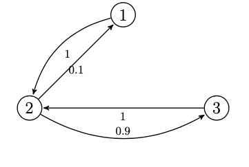
\[\begin{bmatrix} 0 & 1 & 0 \\ 0.10 & 0 & 0.90 \\ 0 & 1 & 0 \\ \end{bmatrix}\]For a DTMC with state space \(\{1,2,3\}\) let P be:
here is the transition diagram:
ex_tpm = np.array([0,1,0,0.1,0,0.9,0,1,0]).reshape(3,3)
la.matrix_power(ex_tpm, 5000)
la.matrix_power(ex_tpm, 5001)
\[\begin{bmatrix} 0.1 & 0 & 0.9 \\ 0.0 & 1 & 0.0 \\ 0.1 & 0 & 0.9 \\ \end{bmatrix}\]For \(P^n\):
\[\begin{bmatrix} 0 & 1 & 0 \\ 0.10 & 0 & 0.90 \\ 0 & 1 & 0 \\ \end{bmatrix}\]For \(P^{2n-1}\):
Thus the pmf of \(X_n\) does not approach a limit. It fluctuates between two pmfs that depend on the initial distribution. The DTMC has no limiting distribution.
Although this DTMC doesn’t have a limiting distribution we observe that if the initial distribution is [0.05, 0.50, 0.45] then solution to the balance equation is unique. Therefore, if that is the inital distribution then PMF of \(X_n\) is [0.05, 0.50, 0.45] \(\forall n \geq 0\). This initial distribution is known as a stationary distribution.
Formally, Def 4. Stationary Distribution:
\[\pi^* = [\pi_1^*, \pi_2^*, ..., \pi_N^*] \ \text{is a stationary distribution if} \\ P(X_0 = i) = \pi_i^* \forall 1 \leq i \leq N \implies \\ P(X_n = i) = \pi_i^* \forall 1 \leq i \leq N, \ n \geq 0\]Formally: Theorem 7, Stationary Distribution
\[\pi^* = [\pi_1^*, \pi_2^*, ..., \pi_N^*] \ \text{is a stationary distribution if and only if it satisfies} \\ \pi^* = \pi^*P \\ and \sum_j \pi^* = 1\]Note that, if a limiting distribution exists it is also a stationary distribution. Skipping a formal proof, we can emperically check this using our running example.
ex_inidist = np.array([0.23076923, 0.35897436 ,0.41025641]).reshape(1,3)
for i in range(15):
  dtmc.pmf(ex_inidist, ex_tpm, i)
  print(dtmc.pmf_)
which gives:
\[[[0.23076923 0.35897436 0.41025641]] \\ [[0.23076923 0.35897436 0.41025641]] \\ [[0.23076923 0.35897436 0.41025641]] \\ [[0.23076923 0.35897436 0.41025641]] \\ [[0.23076923 0.35897436 0.41025641]] \\ [[0.23076923 0.35897436 0.41025641]] \\ [[0.23076923 0.35897436 0.41025641]] \\ [[0.23076923 0.35897436 0.41025641]] \\ [[0.23076923 0.35897436 0.41025641]] \\ [[0.23076923 0.35897436 0.41025641]] \\ [[0.23076923 0.35897436 0.41025641]] \\ [[0.23076923 0.35897436 0.41025641]] \\ [[0.23076923 0.35897436 0.41025641]] \\ [[0.23076923 0.35897436 0.41025641]] \\ [[0.23076923 0.35897436 0.41025641]] \\\]Therefore, if we use the limiting distribution as the initial distribution, i.e [0.23076923, 0.35897436, 0.41025641], we observe that it behaves as the stationary distribution.
Appendix
import numpy as np
import numpy.linalg as la

class DTMC:
    """
    A Discrete Time Markov Chain class

    """
    def __init__(self):
        self.pmf_ = None
        self.conditional_pmf_ = None
        self.ocm_ = None
        self.complementary_conditional_cdf_ = None
        self.absorption_prob_ = None

    def pmf(self, inidist, ptm, interval):
        """
        Computes the Probability Mass Function of the DTMC for the given interval

        Arguments:
        inidist = initial distribution of the DMTC
        ptm = probability transition matrix of the DTMC
        interval = discrete time interval at which PMF is required
        """
        self.pmf_ = np.dot(inidist, la.matrix_power(ptm, interval))

    def conditional_pmf(self, ptm, interval):
        """
        Computes the conditionl Probability Mass Function of the DTMC for the given interval, conditioned on initial state

        Arguments:
        ptm = probability transition matrix of the DTMC
        interval = discrete time interval at which conditional PMF is required
        """
        self.conditional_pmf_ = la.matrix_power(ptm, interval)

    def occupancy_time(self, ptm, interval):
        """
        Computes the occupancy matrix of the DTMC

        Arguments:
        ptm = probability transition matrix of the DTMC
        interval = discrete time interval till which summation is required
        """
        ocm_list = []
        for i in range(interval+1):
            ocm_list.append(la.matrix_power(ptm, i))
        self.ocm_ = sum(ocm_list)

    def complementary_conditional_cdf(self, ptm, fpt_state, n = None):
        """
        Computes the conditional CDF of first passage time T

        Arguments:
        ptm = probability transition matrix of the DTM
        fpt_state = first passage time state being analyzed
        """
        ptm_sub = np.delete(np.delete(ptm, fpt_state, 0), fpt_state, 1)
        e = np.ones((ptm_sub.shape[0], 1))
        self.complementary_conditional_cdf_ = np.dot(la.matrix_power(ptm_sub, n), e)

    def absorption_prob(self, ptm, fpt_state, n = 5000):
      """
      Computes the conditional CDF of first passage time T

      Arguments:
      ptm = probability transition matrix of the DTM
      fpt_state = first passage time state being analyzed
      n = infinity
      """
      self.complementary_conditional_cdf(ptm, fpt_state, n = 5000)
      self.absorption_prob_ = 1 - self.complementary_conditional_cdf_