Measures hidden in Probability
Connecting the links between Measure Theory and Probability Theory can help open up a new perspective. This perspective can be useful while trying to think about probability in an abstract manner i.e as a quantity we would like to distribute across a region in space.
First let’s briefly look at the experimental view point of probability.
Experimental Viewpoint (EV)
Exepriment, Sample Space: Traditionally, we use the notion of an experiment to define a sample space. We consider an experiment to be non-deterministic but it’s set of all outcomes to be known. This known set of all possible outcomes is defined as the sample space. Common notations are \(S, \Omega\). Naturally, \(S^c = \emptyset\).
Event \((E)\): Any subset of the sample space is defined as an event. If the outcome of our experiment ends up in an event \(E\), then we can deterministically state that \(E\) has occured.
Probability: Here, probability is defined using an axiomatic approach. We assume that for each event in the sample there exists a probability, \(P(E)\). Thereafter, we assume that each of these probabilities satisy a set of intuitive axioms. The three axioms are as follows:
- \[P(S) = 1\]
- \[0 \geq P(E) \leq 1\]
- For mutually exclusive events, \(P(\bigcup_{i}E_i) = \sum_{i}P(E_i)\) - countable additivity.
Now, probability is formally defined as the limiting proportion of time \(E\) occurs:
\[P(E) = lim_{n \rightarrow \inf} \frac{n(E)}{n}\]Due to the above defined axioms, we know for a fact that this value converges to a constant.
Random Variable: is defined as “a real valued function on the sample sapce” [3] .
Measure based Viewpoint
To think about probability in terms of measure, first we would like to have a function that maps a value from a given set to another set. i.e \(\mu: X \rightarrow number \ni X \in R^n and \ number \in [0,\inf]\) adhering to certain properties.
However, this is not possible due to the presense of certain strange subsets in \(R^n\). Therefore, instead of describing this function for all subsets of \(R^n\) we constrain it to a certain class of subsets within \(R^n\). This class is known as \(\sigma\)-algebra.
Onto some terminology,
\(\sigma\)-algebra: Let \(X\) be a nonempty set, an algebra is a non empty collection of subsets of X that is closed under finte unions and complements. A \(\sigma\)-algebra is an algebra that is closed under countable unions.
Measure, Measureable Space, Measureable Sets: - Now, a measure for a set \(X\) equipped with a \(\sigma\)-algebra \(\mathcal{M}\), i.e \((X,\mathcal{M})\) - measureable space, is a function \(\mu: \mathcal{M} \rightarrow [0,inf]\) such that:
- i. \(\mu(\emptyset) = 0\)
- ii. Countable additivity for a sequence of disjoint sets in \(\mathcal{M}\).
\((X,\mathcal{M},\mu)\) is called a measure space. Set’s in \(\mathcal{M}\) are called measureable sets, \(E \in \mathcal{M}\).
Now, a small detour to build some intuition.
Let’s suppose we are 4 years of age and are given a box full of books. We are now asked to count the no. of books in that box. How do we do it? We simply open the box, think of each book as a constant value say natural number 1 and add up all occurences of this constant. Using measure-theoretic notions, we can define this process formally as follows: say we have \((X,\mathcal{M})\), \(f:X \rightarrow 1\), \(\mu(E) = \sum_{x \in E} f(x)\) where \(E \in \mathcal{M}\). This measure, is called a counting measure. Pretty intuitive.
Now, say we were asked how many books in the box have an orange cover. How do we count that? This time, we assign the constant value 1 to only those books that have an orange cover and 0 to all other books. Formally, for the same setting say we have some \(x_0 \in X\) then \(f(x_0) = 1\) and \(f(x) = 0 \forall x \neq x_0\). Then \(\mu\) is called a point mass or Dirac measure.
Now, how can we define probability using this framework?
Probability: can simply be defined as a special type of measure. Let \((\Omega, \mathcal{B})\) be a measureable space. Let \(A\) be the set’s in \(\mathcal{B}\). Let \(P\) be a function \(P: \mathcal{B} \rightarrow R\) such that:
- \(P(A) \geq 0 \forall A \in \mathcal{B}\).
- \[P(\Omega) = 1\]
- If \(\{A_i\}_1^n\) are disjoint set’s then: \(P(\bigcup_{i}A_i) = \sum_i(A_i)\) - finite additivity. (Countable additivity is already satisfied in the def. of a measure. Note that, countable additivity implies finite additivity).
This \(P\) is known as a probability measure. Observe that, Event from the EV definition is now simply a measureable set.
Measureable real valued function\(f\): If \((X,\mathcal{M})\) and (\(Y,\mathcal{N}\)) are measureable spaces, a mapping \(f: X \rightarrow Y\) is called measureable if \(f^{-1} (E) \in \mathcal{M} \ \forall \ E \in \mathcal{N}\). When \(f: X \rightarrow R\), then it is called a measureable real valued function. Here, \(f^{-1}\) stand for pre-image.
This measureable real valued function is the EV’s Random Variable equivalent.
Now let’s use this notion and an example to rethink a few things. Say we have an experiment where we toss 3 fair coins simultaneously. Let our random variable \(V\) denote the no. of heads in this experiment. Depending on the throw it can take on any of these 4 values i.e \(Val(V) = \{0,1,2,3\}\). Therefore, there is a probability measure assosiated with this random variable. But how do we specify it? One way to specify it is to directly state the probability of each value this random variable can take, i.e \(P(V = v)\). This is simply the Probability Mass Function. Similarly, we can also define the CDF and PDF (for continous R.V’s).
Therefore, these functions (CDF, PMF, PDF) are used to specify the probability measure assosiated with a random variable. Hence, they are not probabilities in the abstract sense rather representations of the abstract notion of probability assosiated with a Random Variable.
Highly recommend [1] (for an intuitive understanding) and [2] (for a formal understanding) as further reading.
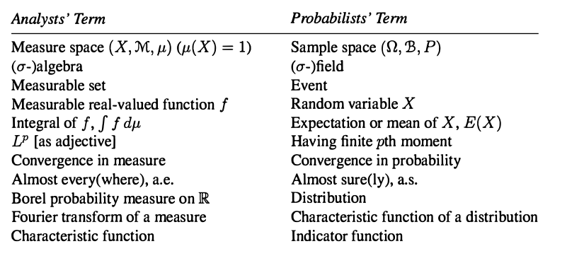
Below is a lovely picture from [2] mapping the similarites mentioned above:
References
[1] - Betancourt, Probability Theory
[2] - Folland, G. B. 1999. Real Analysis: Modern Techniques and Their Applications. New York: John Wiley; Sons, Inc.
[3] - Ross, S.M., 2006. A first course in probability (Vol. 7). Upper Saddle River, NJ: Pearson Prentice Hall.