Fraud Transactions: Classification and Stochastic Modeling

This post encompasses a classification model to predict fraudulent transactions and a continuous time stochastic model to understand the transient distribution, occupancy times and limiting behaviour.

Introduction

Data set is from here. In brief, it containts credit card transactions for 2 days where 0.172% of all transactions are fraudulent. There are 29 features of which 28 are linear Prinicpal components and one amount (Therefore all \(\in R\) ) with names masked for confidentiality. Target is a bernoulli random variable which takes on two distinct values 0 - for non-fraudulent transaction and 1 - for fraudulent transaction.

Modeling - Classification

Preprocessing

• Check for null values.

#Check for null values
sum(data.isna().sum())

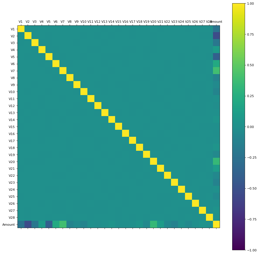
• Since the features are P.C’s there will be no correlation amidst them. (Quick reminder: This is because in PCA, while solving the optimization problem to maximize projected variance one of the two constraints we use is \(u_i^Tu_j = 0, i \neq j\). where \(u\) denotes the basis of the subspace onto which we are projecting. Intutively, the reason we do is that is because we want to select basis’s that capture most of the variation.) To re-confirm this we can plot a correlation matrix.

As expected there is no correlation between PC’s. There appears to be a negative correlation between amount and V2,V5 but let us ignore that for the time being.

• Scale the values in order to avoid one factor to dominate.

#Scale the columns
scaler = MinMaxScaler()
scaler.fit(data.iloc[:,1:30])
data1 = pd.DataFrame(scaler.transform(data.iloc[:,1:30]), columns = data.columns[1:30])
data1['response'] = data.iloc[:, 30:31]

• We can define two half planes and solve a greedy - recursive binary tree problem to find the \(\underset{p,s}{argmin} \ \forall \ p\) (where p stand for predictor and s for cutpoint within that predictor) to find the predictors that explain our response the best or alternatively, we could proceed to build our model with all the features, evaluate performance using area under the ROC curve, then depending on the results evaluate how the predictors explain our response. Let us proceed with the alternative approach.

Classification - I

Modeling \(D\) using Random forest with 5-fold cross validation and evaluating using area under ROC curve since it is a biased classification problem.

#classification-I
X = np.array(data1.iloc[:, 1:29])
y = np.array(data1.iloc[:, 29:30])
#creating a scoring metric
roc = make_scorer(roc_auc_score)
#random forest
clf = RandomForestClassifier(n_estimators=200)
#5-fold cv
rf_score = cross_val_score(clf, X, y, scoring=roc,
                cv=5)
def mean(l):
    return(sum(l)/len(l))
mean(rf_score)

Oversampling

Since this is a biased classification we could either tweak the cost function to penalize incorrectly classifying the minority class more,

Or alternatively oversample using with something like \(SMOTE^{[1]}\). In brief, The SMOTE approach works as follows. i.) For each minority instance, its k nearest neighbors belonging to the same class are determined. ii.) Then, depending on the level of oversampling required, a fraction of them are chosen randomly. iii.) For each sampled example-neighbor pair, a synthetic data example is generated on the line segment connecting that minority example to its nearest neighbor. The exact position of the example is chosen uniformly at random along the line segment. iv.) These new minority examples are added to the training data, and the classifier is trained with the augmented data.

Below is a quick python implementation:

#SMOTE
def SMOTE(data, response_name, minority_encoding, percent_match, K):
#store the K - nearest neighbours of all minority classes in one list
    data_mino = np.array(data.loc[:, data.columns != response_name][data[response_name] == minority_encoding])
    large = 1000000
    dist = np.linalg.norm(data_mino - data_mino[:,None], axis=-1)
    np.fill_diagonal(dist, large)
    nearest_neigh = list()
    for repeat in range(K):
        nearest_list = dist.argmin(axis = 1)
        nearest_neigh.append(nearest_list)
        row_index = [i for i in range(len(nearest_list))]
        replace_index = list(zip(row_index, nearest_list))
        for i in replace_index:
            dist[i] = large
    k_nearest_neigh = list(zip(*[nearest_neigh[i] for i in range(K)]))
#Compute N
    N = int((percent_match*data.shape[0])/data_mino.shape[0])
    print(N)
#Generate the synthetic samples
    index = 0
    synthetic = np.zeros(((N*data_mino.shape[0]), (data_mino.shape[1])))
    while N != 0:
        for i in range(data_mino.shape[0]):
            nn = random.randrange(0, K)
            dif = data_mino[k_nearest_neigh[i][nn]][:(data_mino.shape[1])] - data_mino[i][:(data_mino.shape[1])] #DIF
            gap = random.uniform(0, 1)
            synthetic[index] = data_mino[i][:(data_mino.shape[1])] + (gap * dif)
            index += 1
        N -= 1
    new_col = np.repeat(1, synthetic.shape[0]).reshape(synthetic.shape[0], 1)
    final = np.append(synthetic, new_col, axis = 1)
    return(final)

In this implementation we skip randomly sampling a fraction of the minority indices as we seek to use all of the minority samples.

#Oversampling minority from original matrix
s = time.time()
synthetic = SMOTE(data.iloc[:,1:31], 'Class', 1, 0.50, 5)
f = time.time()
print((f-s)/60)

#Oversampled dataset
temp = np.vstack((data.iloc[:,1:31], synthetic))
np.random.shuffle(temp)
temp = pd.DataFrame(temp)
#Scaling the oversampled dataset
scaler.fit(temp.iloc[:,0:29])
data2 = pd.DataFrame(scaler.transform(temp.iloc[:,0:29]), columns = data.columns[1:30])
data2['response'] = temp.iloc[:, 29:30]

Also note that, oversampling was performed on the non-scaled original dataset to maintain symmetry of the original feature space.

Classification - II

Re-classifying after oversampling the data in the same format as before.

#classification-II
X_2 = np.array(data2.iloc[:, 1:29])
y_2 = np.array(data2.iloc[:, 29:30])
#5-fold cv
rf_score_2 = cross_val_score(clf, X_2, y_2, scoring=roc,
                cv=5)

Results

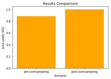
Comparing both the results:

Stochastic Modeling

One way to model this problem as a CTMC is to think that transactions are not-fraudulent for an Exp(\(\mu\)) amount of time and then fraud happens. Once there is fraud, the transactions are fraudulent for an Exp(\(\lambda\)) amount of time and is independent of the past.

In that case, \(\{X(t), t\geq0\}\) is a continuous time stochastic process where \(X(t)\) is the state of the process at time \(t\) with a state space \(\{0,1\}\) (0:non-fraudulent, 1:fraudulent). The sojourn time in state 0 is the non-fraud time which is an Exponential random variable with parameter \(\mu\) hence, \(r_0 = \mu\) and \(p_{0,1} = 1\) since a transaction could just fail. Similarly, \(r_1 = \lambda\) and \(p_{1,0} = 1\). Therefore, the Rate matrix is

\[R = \begin{bmatrix} 0, \mu \\ \lambda, 0 \end{bmatrix}\]

Now, one way to find out the above parameters: i.) Think of reaching state \(i\) from \(j\) where \(i,j \in \{0,1\}\) as one run of an exponential R.V and compute the amount of time our CTMC stays in a particualar state for each such run ii.) Compute \(E[X]\) and then iii.) compute \(\frac{1}{E[X]}\)

data3 = data.loc[:, ['Time', 'Class']]
time = data3.loc[:,'Time'].tolist()
state = data3.loc[:, 'Class'].tolist()

#Getting time spend in state 0 for each instance
indices = [i for i, x in enumerate(state) if x == 1]
exp_time_0 = []
for i in range(len(indices)):
    if i ==0:
        exp_time_0.append(time[indices[i]])
    else:
        exp_time_0.append(time[indices[i]] - time[indices[i-1]])

mu = 1/mean(exp_time_0)

#Getting time spend in state 1 for each instance
len(set(indices)) #fraud happens at all unique intervals
exp_time_1 = []
for i in range(len(indices)):
        exp_time_1.append(time[indices[i]+1]-time[indices[i]])

lamda = 1/mean(exp_time_1)

References

1. Chawla, N. V. (2002). SMOTE: Synthetic Minority Over-sampling Technique. Journal of Artificial Intelligence Research.

2. Hastie, T., Tibshirani, R., & Friedman, J. H. (2004). The elements of statistical learning: Data mining, inference, and prediction.

3. Modeling and Analysis of Stochastic Systems, by Vidyadhar G. Kulkarni, Taylor & Francis, 2009.