Regularized Regression

This post entails an elementary implementation of two common regularization techniques namely Ridge and Lasso in the context of Regression in R using a housing dataset.

When we try to fit a higher order polynomial in cases where there are a lot of independent variables we notice that our model tends to overfit (i.e have high variance). This is because, given a lot of dimensions it is not feasible to have training observations covering all different combinations of inputs. More importantly, it becomes much harder for OLS assumptions to hold ground as the no. of inputs increase. In such cases when can use regularization to control our regression coefficients and in turn reduce variance.

Ridge Regression

Ridge Regression is particularly useful in cases where we need to retain all inputs but reduce multicolinearity and noise caused by less influential variables.

Therefore, the objective in this case is predict the target variable considering all inputs.

Mathamatically, it can be defined as:

Minimize:

\[\sum_{i=1}^{n}({y_i}^2 -\hat{y}^2_i)+\lambda||w||^2_2\]

where,

Residual sum of squares = \(\sum_{i=1}^{n}({y_i}^2-\hat{y}^2_i)\)

Tuning parameter = \(\lambda\)

L2 norm = \(\||w||^2_2\) i.e \(\sum_{i=1}^{n}w^2_i\)

Geometric intution:

The 2D contour plot below provies intution as to why the coefficients in ridge shrink to near zero but not exactly zero as we increase the tuning parameter(\(\lambda\)).

In the above figure RSS equation has the form of an elipse (in red) and the L2 norm for 2 variables is naturally the equation of a circle (in blue). We can observe that their interaction is when \(\beta_2\) is close but not equal to 0.

First, let us load the packages we’d be needing:

#Libraries to be used
library(glmnet) #regularized regression package
library(ggplot2) #for plotting
library(caret) #hot one encoding
library(e1071) #skewess function
library(gridExtra) #grid mapping

Preprocessing

#Importing King county house sales dataset locally
getwd()
setwd("/Users/apple/Google Drive/github/Regularization")
data = read.csv('kc_house_data.csv')
data = subset(data, select = -c(id, date))
data$floors = as.character(data$floors)
data$zipcode = as.character(data$zipcode)
str(data)
dim(data) #21613 x 19
sum(is.na(data)) #No missing data

#Plotting histograms to see distribution of all numeric variables

#gather all non charecter features
feature_class = sapply(colnames(data),function(x){class(data[[x]])})
numeric_features = names(feature_class[feature_class != "character"])
numeric_features

#Plotting using ggplot and fixing grid using gridExtra
dist_list = list()
for (i in numeric_features){
  dist_list[[i]] = ggplotGrob(ggplot(data = data, aes_string(x = i)) + geom_histogram(aes(x = data[i])) + theme_grey())
}

grid.arrange(dist_list[[1]],dist_list[[2]],dist_list[[3]],dist_list[[4]], dist_list[[5]],
             dist_list[[6]],dist_list[[7]],dist_list[[8]],dist_list[[9]],dist_list[[10]],
             dist_list[[11]], dist_list[[12]], ncol=3)

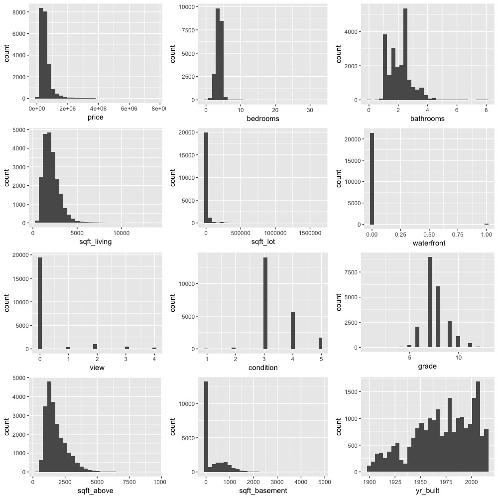
From the above image we can observe that most of the variables are not normally distributed and highly skewed. To get rid of the skewness and to transform to normality we can apply a power transformation such as log.

#Removing skew for all numeric features using a power transformation (log) and hot one encoding categorical variables

# determine skew for each numeric feature
skewed_feats = sapply(numeric_features, function(x) {skewness(data[[x]])})
skewed_feats
#remove skew greater than 1
rem_skew = skewed_feats[skewed_feats>1]
rem_skew
for (i in names(rem_skew)){
  data[[i]] = log(data[[i]]+1) # +1 as we have many 0 values in many columns
}
head(data)

#hot one encoding
categorical_feats = names(feature_class[feature_class == "character"])
categorical_feats
dummies = dummyVars(~., data[categorical_feats]) #from library caret
categorical_1_hot = predict(dummies, data[categorical_feats])

#Create master file and perform training-testing split

#Combining files
master_data = cbind(data[numeric_features], categorical_1_hot)

#Creating a training and testing split
l = round(0.7*nrow(master_data))
set.seed(7)
seq_rows = sample(seq_len(nrow(master_data)), size = l)
data_train = master_data[seq_rows,]
data_test = master_data[-seq_rows,]

Implementation

Points to note:

1. glmnet package trains our model for various values of \(\lambda\)

2. It provides a built-in option to perform k-fold CV.

3. It standardizes predictor variables

4. It doesn’t accept the regular formula method (y ~ x) instead we need to supply an input matrix

(read the documentation for more info) link

Flow:

1. Train model and perform k-fold cross validation to pick the \(\lambda\) value that minimizes MSE

2. Use this \(\lambda\) value to build a model on the entire training set

3. Use the model from 2. to predict house prices on the test set

4. Compare predictions with actual house prices and evaluate fit

#create matrices
data_train_x = as.matrix(data_train[,2:93])
data_train_y = as.matrix(data_train$price)
data_test_x = as.matrix(data_test[,2:93])
data_test_y = as.matrix(data_test$price)

#1. k-fold cv (k = 10 by default)
ridge_cv = cv.glmnet(
  x = data_train_x,
  y = data_train_y,
  alpha = 0 #0 for ridge
)
plot(ridge_cv)

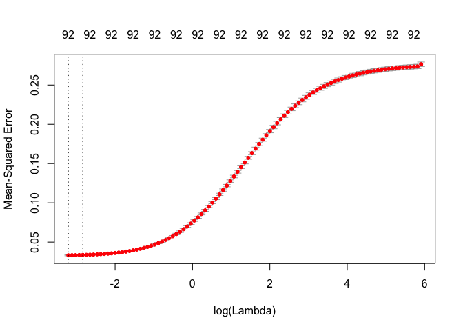
From the plot we can observe that MSE increases once log(\(\lambda\)) is greater than -2. The first dotted line is the \(\lambda\) value with minimum MSE and the second dotted line is the \(\lambda\) value at one standard error from minimum MSE.

min(ridge_cv$cvm) #lowest MSE
ridge_cv$lambda.min #lambda for lowest MSE
min = ridge_cv$lambda.1se #selecting the 1st se from lowest

#2. Final model
#visualization
ridge = glmnet(
  x = data_train_x,
  y = data_train_y,
  alpha = 0
)
plot(ridge, xvar = "lambda")
abline(v = log(ridge_cv$lambda.1se), col = "red", lty = "dashed") #lambda value we picked

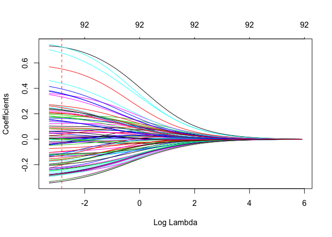
In the above plot the red dotted line is the log(\(\lambda\)) value that gives us the lowest MSE.

#building model using the seleceted lambda value
ridge_min = glmnet(
  x = data_train_x,
  y = data_train_y,
  alpha = 0, lambda = min
)
#Visualizing important variables

#function to return dataframe of coefficents without an intercept
coefficents = function(coefi, n){
  #coefi -> is the beta output of glmnet function
  #n -> is the desired number of features to be plotted
  #returns features coerced with values ordered in desc by abs value
  coef_v = as.matrix(coefi)
  as.data.frame(coef_v)
  colnames(coef_v)[1] = 'values'
  coef_f =  as.data.frame(dimnames(coef_v)[[1]])
  coef_final = cbind(coef_f,coef_v)
  colnames(coef_final)[1] = 'features'
  coef_final = coef_final[order(-abs(coef_final$values)),]
  coef_final$values = round(coef_final$values, 2)
  coef_final = coef_final[1:n,]
  return(coef_final)
}

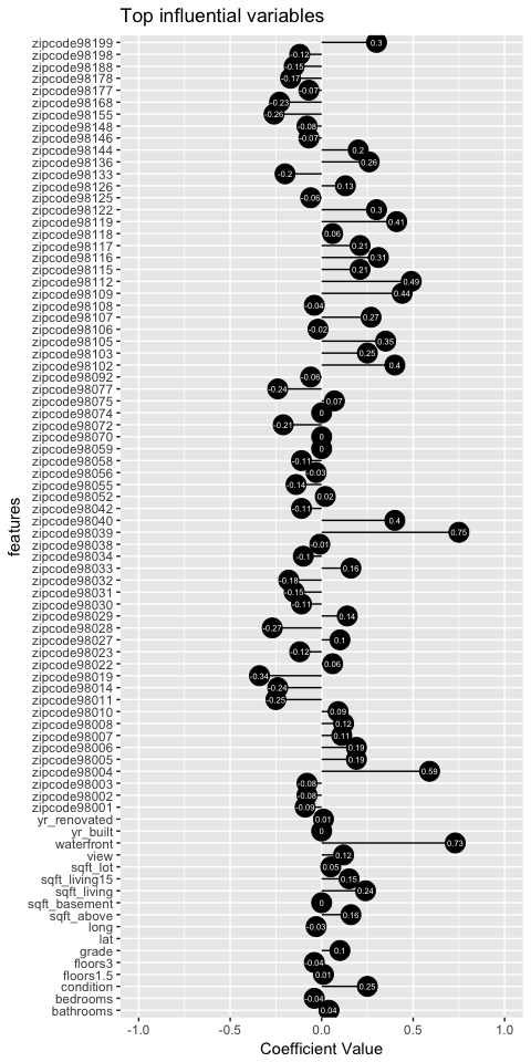
ggplot(coefficents(ridge_min$beta, 25), aes(x=features, y=values, label=values)) +
  geom_point(stat='identity', fill="Black", size=6)  +
  geom_segment(aes(y = 0,
                   x = features,
                   yend = values,
                   xend = features),
               color = "Black") +
  geom_text(color="white", size=2) +
  labs(title="Top 25 influential variables", y = 'Coefficient Value') +
  ylim(-1, 1) +
  coord_flip()

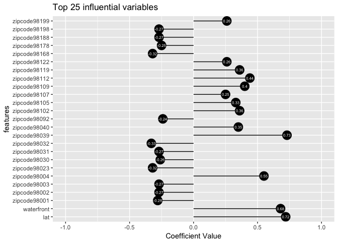
The above plot displays the top 25 influential variables and their coefficient values. Now, we will use our model to predict house price and assess the quality of fit by computing the \(r^2\) value.

#predicting on test set
y_pred = predict(ridge_min, data_test_x)
#function to compute total sum of squares
r_sq = function(y, pred_y){
  #y -> Actual value of y in the test set
  #pred_y -> predicted y value
  tss = sum((y - mean(y))^2)
  rss = sum((pred_y - y)^2)
  return(reslut = 1 - (rss/tss))
}

r_sq(data_test_y, y_pred) #0.8841862

Therefore, our model accounts for 88.4% of the variability in the training data.

As mentioned earlier, Ridge regression is used in cases where we would like to retain all our features while reducing noise caused by less influential features. In case, we would like to make predictions by reduce the number of features in our model to a smaller subset then Lasso regression is used.

Lasso Regression

Objective in this case is predict the target variable considering a subset of inputs (i.e seek a sparse solution).

Mathamatically, it can be defined as:

Minimize:

\[\sum_{i=1}^{n}({y_i}^2 -\hat{y}^2_i)+\lambda||w||_1\]

where,

Residual sum of squares = \(\sum_{i=1}^{n}({y_i}^2-\hat{y}^2_i)\)

Tuning parameter = \(\lambda\)

Geometric intution:

The 2D contour plot below provides intution as to why the coefficients in lasso shrink to exactly zero instead of near zero like ridge.

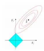
In the above figure RSS equation has the form of an elipse (in red) and the L1 norm for 2 variables has the shape of a diamond (in blue). We can observe that their interaction is at \(\beta_2\) = 0. This provides intution as to why lasso solutions are sparse. Moreover, as we move to higher dimensions instead of a diamond L1 norm has the shape of a rhomboid which due to it’s ‘pointy’ nature has a greater probability of contact with the RSS equation.

As before \(\lambda\) plays the role of a tuning parameter but in this case, as it’s increased, it pushes some of the insignificant features to zero.

Implementation

As, we have performed the necessary preprocessing we can start the implementaton and our flow will be exatly like before:

1. Train model and perform k-fold cross validation to pick the \(\lambda\) value that minimizes MSE

2. Use this \(\lambda\) value to build a model on the entire training set

3. Use the model from 2. to predict house prices on the test set

4. Compare predictions with actual house prices and evaluate fit

#1. k-fold cv (k = 10 by default)
lasso_cv = cv.glmnet(
  x = data_train_x,
  y = data_train_y,
  alpha = 1 #1 for lasso
)
plot(lasso_cv)

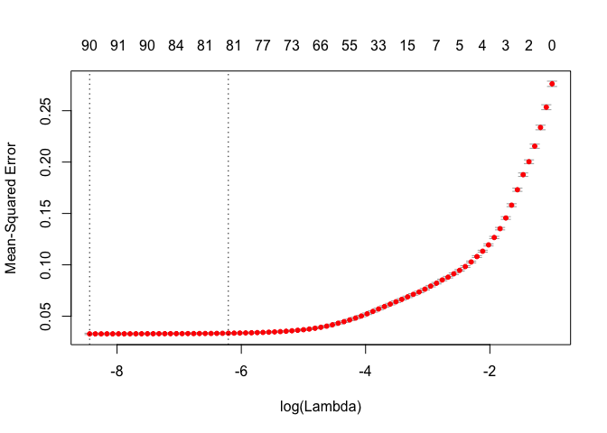
As before, the first dotted line is the \(\lambda\) value with minimum MSE and the second dotted line is the \(\lambda\) value at one standard error from minimum MSE. Also notice how our features decrease the \(\lambda\) value increases.

min(lasso_cv$cvm) #lowest MSE
lasso_cv$lambda.min #lambda for lowest MSE
min_l = lasso_cv$lambda.1se #selecting the 1st se from lowest

#2. Final model
#visualization
lasso = glmnet(
  x = data_train_x,
  y = data_train_y,
  alpha = 1
)
plot(lasso, xvar = "lambda")
abline(v = log(lasso_cv$lambda.1se), col = "red", lty = "dashed") #lambda value we picked

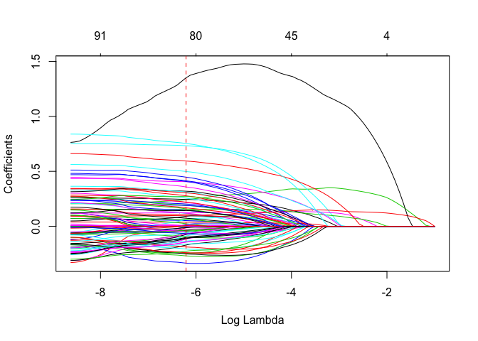
Notice how the coefficient path is significantly different in ridge and lasso. We can observe that in ridge the coefficients mostly flock together but in this case they are all over the place. This is because, ridge distributes weights of the features to keep its \(w^2\) value low (and hence the cost function). A downside of this is that the individual impact of features will not be very clear.

#building model using the seleceted lambda value
lasso_min = glmnet(
  x = data_train_x,
  y = data_train_y,
  alpha = 1, lambda = min_l
)

#number of non zero coeff
length(lasso_min$beta[lasso_min$beta!=0]) #82

The obove plot shows all the remaining influential variables and their coefficient value.

Now, predicting results and model assesment.

#predicting lasso on test set
y_pred_l = predict(lasso_min, data_test_x)
#computing r_squared
r_sq(data_test_y, y_pred_l)

Our model holds slightly better than ridge accounting for 88.5% of the variability. However, notice that this prediction was with 82 features instead of 92 like in ridge.

Conclusion

In this post we looked at the intution behind ridge and lasso regression along with it’s implementaton in R using the glmnet package. Regularization is particularly useful while dealing with bias-variance tradeoff.

Entire code can be found on my github.

References

Giersdorf, J. (2017). Analysis of Feature-Selection for Lasso Regression Models. link