Nonlinear Programming: Methods for Unconstrained Optimization

Nonlinear Optimization sits at the heart of modern Machine Learning. For a practioner, due to the profusion of well built packages, NLP has reduced to playing with hyperparameters. This post briefly illustrates the ‘Hello World’ of nonlinear optimization theory: Unconstrained Optimization. We look at some basic theory followed by python implementations and loss surface visualizations.

Motivation

• Once we set up a ML problem with a certain hypothesis, it can be solved as an optimization problem.

• Almost, all ML algorithms can be formulated as an optimization problem to find the max/min of an objective function.

Supervised Learning

• \(X \in R^p\), \(Y \in R\).

• Learn a function that is able to predict X at given values of Y.

• Define the residual as \(r_i = L(y_i - f(x_i;\theta))\) where \(L\) is say the squared error loss.

• Set up the goal to find the optimal function as follows (least squares problem):

\[min_\theta f(\theta) = \frac{1}{2N} \sum_{i=1}^N L(y_i, f(x_i,\theta))\]

where \(i\) is defined over the training set.

Semi-Supervised

• Have both labelled and unlabelled data here.

• Common stratergy here is to optimise a standard supervised classification loss on labelled samples

• Along with an additional unsupervised loss term imposed on either unlabelled data or both labelled and unlabelled data.

• These additional loss terms are considered as unsupervised supervision signals, since ground-truth label is not necessarily required to derive the loss values.

• For a 2 class problem with SVM’s is as follows:

\[argmin_f \frac{1}{l}\sum_{i=1}^l max(1-y_if(x_i),0) + \lambda_1||f||^2 + \lambda_2 \frac{1}{u} \sum_{i = l+1}^{l+u} max(1-|f(x)|,0)\]

• Minimize the objective for supervised support vector machines with hinge function and the average hat loss for unlablled instances.

Unsupervised Learning

Clustering problem

• Given \(D \in R^{n*d}\), we want to partition it into \(K\) clusters.

• Using a scoring function such as SSE, we can set up the optimization problem as follows:

\[argmin_{C_1,C_2,...C_K} \sum_{i=1}^k\sum_{x_j \in C_i} ||x_j - \mu_i||^2\]

where \(\mu\) is a summary statistic of each cluster such as the mean.

Dimensionality Reduction

• \(D \in R^{n*d}\) where each row is spanned by \(d\) standard basis vectors i.e \(e_1,e_2...e_d\)

• Project points from our Dataset \(D\) onto a lower dimensional subspace \(A\) in such a way that we capture most of the variation in our data.

• One way to select an optimum basis among all basis would be to set this up as a variance maximation problem i.e choose a basis that maximizes the projected variance.

\[Max \ \sigma^2 = w^T \Sigma w \\ s.t \ i.) w^Tw = 1 \\ ii.) \ u_i^Tw = 0 \ \forall \ i \in \{1,2...,j-1\}\]

Unconstrained Optimization Basics

Basic Definitions:

• Continuous Optimization: Variables ∈ R.

• Unconstrained Optimization: Minimize OF that depends on real variables with no restrictions.

\[min_\theta f(\theta)\]

where \(\theta \in R^n, n\geq 1, f: R^n \rightarrow R\) is a smooth function.

• Constrained Optimization: Explicit bounds on the variables. Have equality, inequality. Eg: Norms. (Not covered in this post.)

Basic Theory

• Global Minimizer: A point \(\theta^*\) is a global minimizer if \(f(\theta^*) \leq f(\theta)\) for all \(\theta\).

• Weak Local Minimizer: A point \(\theta^*\) is a weak local minimizer if there is a neighbourhood \(N\) of \(\theta^* \ni f(\theta^*) \leq f(\theta) \forall x \in N\).

• Strict Local minimizer: \(f(\theta^*) < f(\theta)\) (outright winner) with \(\theta \neq \theta^*\)

Picture

• Necessary condition: Min criteria parameter must satisfy to be of interest. But just satisying it is not enough.

• FONC: If \(\theta^*\) is a local min and $f$ is continuously differentiable in an open neighborhood of \(\theta^*\), then \(\nabla f(\theta^*) = 0\)

  • Points satisfying \(\nabla f(\theta^*) = 0\) are stationary points: min, max, saddle points.
  • \(\nabla f(\theta^*) = 0\) guarantees global minimality of \(\theta^*\) if f is convex.

• SONC: If \(\theta^*\) is a local min and \(\nabla^2 f\) exists and is continuous in an open neighborhood of \(\theta^*\), then \(\nabla f(\theta^*) = 0\) and \(\nabla^2 f(\theta^*)\) is positive semi deifinite.

• Sufficient condition: If this is met, can call it a min.

• SOSC: \(\nabla f(\theta^*) = 0\) (FONC) and \(\nabla^2 f(\theta^*)\) is p.d then \(\theta^*\) is a strict local minimizer.

Fundamental approach to optimization

General idea:

• Start at a \(\theta_0\), generate a sequence of iterates \(\{\theta_k\}_{k=0}^{\inf}\) that termintates when it seems a reasonable solution has been found.

• To move from one iterate to another, we use information of \(f\) at \(\theta_k\) or from earlier.

• Want \(f(\theta_k) < f(\theta_{k+1})\)

Fundamental Stratergy:

• Two fundamental stratergies, for moving from \(\theta_k\) to \(\theta_{k+1}\).

  • Line Search Fix direction, identify step length.
    • Algorithm chooses a direction \(p_k\), search along \(p_k\) from \(\theta_k\) to find a new \(\theta_{k+1} \ni f(\theta_{k+1}) < f(\theta_{k})\).
    • How far to move along this direction?:
      1) Exactly solve 1-d min problem: \(min_{\alpha>0}f(\theta_k + \alpha p_k)\)
      2) Generate limited no. of trial length steps.
    • How to choose search direction? Choose guaranteed descent direction. (Add Proofs).
  • Trust Region Choose distance, then find direction.
    • At \(\theta_k\), construct a model function \(m_k\) (using taylors theorem) whose behaviour at \(\theta_k\) is similar to actual \(f\).
    • We find the direction $p$ to move in by solving subproblem \(min_p \ m_k(\theta_k + p)\)
    • Restrict search for minimizer of \(m_k\) to some region around \(\theta_k\) because \(m_k\) not a good approximation of \(f\) if \(\theta\) is far away.

    • Usually, trust region is a ball $$

      p

      _2 \leq \Delta$$, ellipse or box depending on norm.

    • If candidate solution not found, trust region too large, shrink \(\Delta\) and repeat.

Exploring Line Search

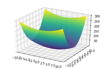
In this post, we use the below two quadratic functions with respective loss surface for implementation and visulization.

• \[x_0^2 - 2.0 x_0 x_1 + 4 x_1^2\]

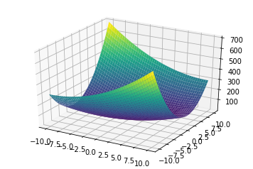
• \[0.5x_0^2 + 2.5x_1^2\]

Preprocessing

We use the SymPy library in python to generate equations in a symbolic manner. Thereafter, create some functions to preprocess these equations in python interpretable variables. We also, create some functions to plot the loss surface and contours.

import numpy as np #arrays
from numpy import linalg as LA #Linear Algebra
import matplotlib.pyplot as plt #plotting
import sympy #symbolic computing package
from sympy.utilities.lambdify import lambdify #convert sympy objects to python interpretable

##################################################
# CREATING FUNCTIONS USING SYMPY
##################################################

#Create functions using SymPy
v = sympy.Matrix(sympy.symbols('x[0] x[1]'))                    #import SymPy objects

#create a function as a SymPy expression
f_sympy1 = v[0]**2 - 2.0 * v[0] * v[1] + 4 * v[1]**2           #first function
print('This is what the function looks like: ', f_sympy1)

f_sympy2 = 0.5*v[0]**2 + 2.5*v[1]**2                           #second function

f_sympy3 = 4*v[0]**2 + 2*v[1]**2 + 4*v[0]*v[1] - 3*v[0]        #third function

##################################################
# CONVERTING SYMPY EXPRESSIONS INTO REGULAR EXPRESSIONS
##################################################

#Extract Main function
def f_x(f_expression, values):
    '''Takes in SymPy function expression along with values of dim 1x2 and return output of the function'''
    f = lambdify((v[0],v[1]), f_expression)                     #convert to function using lambdify
    return f(values[0],values[1])                               #Evaluate the function at the given value

#Extract gradients
def df_x(f_expression, values):
    '''Takes in SymPy function expression along with values of dim 1x2 and returns gradients of the original function'''
    df1_sympy = np.array([sympy.diff(f_expression, i) for i in v])       #first order derivatives
    dfx_0 = lambdify((v[0],v[1]), df1_sympy[0])                          #derivative w.r.t x_0
    dfx_1 = lambdify((v[0],v[1]), df1_sympy[1])                          #derivative w.r.t x_1
    evx_0 = dfx_0(values[0], values[1])                                  #evaluating the gradient at given values
    evx_1 = dfx_1(values[0], values[1])
    return(np.array([evx_0,evx_1]))

#Extract Hessian
def hessian(f_expression):
    '''Takes in a SymPy expression and returns a Hessian'''
    df1_sympy = np.array([sympy.diff(f_expression, i) for i in v])              #first order derivatives
    hessian = np.array([sympy.diff(df1_sympy, i) for i in v]).astype(np.float)  #hessian
    return(hessian)

##################################################
# FUNCTIONS TO VISUALIZE
##################################################

#Function to create a 3-D plot of the loss surface
def loss_surface(sympy_function):
    '''Plots the loss surface for the given function'''
    #x = sympy.symbols('x')
    return(sympy.plotting.plot3d(sympy_function, adaptive=False, nb_of_points=400))

#Function to create a countour plot
def contour(sympy_function):
    '''Takes in SymPy expression and plots the contour'''
    x = np.linspace(-3, 3, 100)                         #x-axis
    y = np.linspace(-3, 3, 100)                         #y-axis
    x, y = np.meshgrid(x, y)                            #creating a grid using x & y
    func = f_x(sympy_function, np.array([x,y]))
    plt.axis("equal")
    return plt.contour(x, y, func)

#Function to plot contour along with the travel path of the algorithm
def contour_travel(x_array, sympy_function):
    '''Takes in an array of output points and the corresponding SymPy expression to return travel contour plot '''
    x = np.linspace(-2, 2, 100)                         #x-axis
    y = np.linspace(-2, 2, 100)                         #y-axis
    x, y = np.meshgrid(x, y)                            #creating a grid using x & y
    func = f_x(sympy_function, np.array([x,y]))
    plt.axis("equal")
    plt.contour(x, y, func)
    plot = plt.plot(x_array[:,0],x_array[:,1],'x-')
    return (plot)

Algorithms

Classical Newton Method:

Newton’s method is an algorithm for finding a zero of a nonlinear function i.e the points where a function equals 0 (minima).

The basic idea in Newton’s method is to approximate our non-linear function \(f(x)\) with a quadratic (\(2^{nd}\) order approximation) and then use the minimizer of the approximated function as the starting point in the next step and repeat the process iteratively. If \(f \in C^2\) function we can obtain this approximation using Taylor series expansion:

\[f(x) = f(x_0) + (x-x_0)^T \nabla f(x) + \frac{1}{2!} (x-x_0)^T \nabla^2 f(x_0)(x-x_0)\]

Where \(x_0\) is the intitial point about which we try to approximate and \(x\) is the new point. Applying FONC (\(\nabla f(x) = 0\)) to the above equation, we get:

\[x = x_0 - [\nabla^2f(x)]^{-1} \nabla f(x)\]

This \(x\) is a unique global min if the Hessian (\(\nabla^2f(x)\)) is Positive Definite or global min if the Hessian is Positive Semi Definite. If it’s not P.D we can enforce it to be P.D using LM modification. Sometimes, Newton’s method may not possess a descent property, i.e. \(f (x_k+1) \geq f(x_k)\). This is especially true if the initial point \(x_0\) is not sufficiently close to the solution. Therefore, we can use a stepsize (\(\alpha_k\)) to enforce the descent property if Hessian is P.D.

Using this stepsize Newtons method is often writen recurssively as:

\[x_{k+1} = x_k + \alpha_k p_k \rightarrow (N.M)\]

where \(p_k\) is the solution to newton equations such as: \([\nabla^2 f(x_k)]p = -\nabla f(x_k)\). This means that the direction $p_k$ is obtained by solving a system of linear equations and not by computing the inverse of the Hessian. Step size \(\alpha_k\) can be found using exact or numerical line search methods.

Implementation:

####Newton Method
def Newton(sympy_function, max_iter, start, step_size = 1, epsilon = 10**-2):
    i = 0
    x_values = np.zeros((max_iter+1,2))
    x_values[0] = start
    norm_values = []
    while i < max_iter:
        norm = LA.norm(df_x(sympy_function, x_values[i]))
        if norm < epsilon:
            break
        else:
            grad = df_x(sympy_function, x_values[i])
            hessian_inv = LA.inv(hessian(sympy_function))
            p = -np.dot(grad, hessian_inv)
            x_values[i+1] = x_values[i] + step_size*p
            norm_values.append(norm)
        i+=1
    print('No. of steps Newton takes to converge: ', len(norm_values))
    return(x_values, norm_values)

This is what the travel path of the Newton looks like for the two functions:

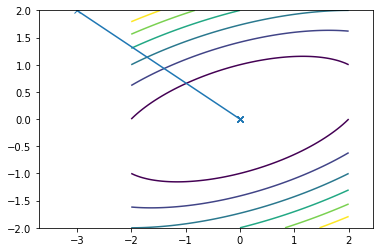
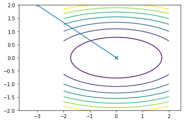
Since, both the functions are quadratic newton convergence in one single iteration.

Pros:

1. Quadratic rate of convergences due to reliance on second order information.

Disadvantages of Newton Method:

1. Can fail to converge or converge to a point that is not a minimum. (Can be fixed with LM modification and line search)

2. Computational costs: if there are n variables, calculating the hessian involves calculating and storing \(n^2\) entries and solving system of linear equations takes \(O(n^3)\) operations per iteration.

To alleviate these cons, we can use methods that reduce the computational cost of Newton but at the expense of slower convergence rates. So, we make a trade-off between costs per iteration (higher for newton) and the no. of iterations (higher for these methods). These methods are based on the newton method but compute the search direction in a different manner. In newton’s method the search direction is computed using

\[p_k = - B_k^{-1} \nabla f(x_k)\]

where \(B_k = \nabla^2f(x_k)\) assuming that the Hessian is Positive Definite. Hence, in order to obtain the search direction \(p_k\) we need to solve a system of linear equations.

In these methods, we instead try to approximate this \(B_k\), the degree of comprise of these methods depends on the degree to which \(B_k\) approximates the Hessian \(\nabla^2f(x_k)\).

Steepest-Descent Method

The idea here is that moving in the direction of the gradient provides steepest increase. Hence, we move in the opposite direction to find the minimum. Therefore, we compute the search direction as:

\[p_k = -\nabla f(x_k)\]

and then use a line search to obtain the transition from \(x^{(k)}\) to another point \(x^{(k+1)}\) at the \(k^{th}\) stage. Therefore, the cost of computing line search is the same as the cost of computing the gradient. This search direction is a descent direction if \(\nabla f(x) \neq 0\).

As mentioned before we are trying to approximate the search direction of the newton method. There are two ways to think about this approximation:

1. Identity Approach: Think of approximating the Hessian, \(B_k\), in Newton using the Identity matrix (I). i.e \(\nabla^2 f \approx I\) to obtain the search direction \(p_k = - \nabla f(x_k)\) for Steepest Descent. The reason for choosing I is motivated by the simplicity of this approach and also because I is Positive Definite hence guaranteeing \(p_k\) to be a descent direction.

2. Taylor Series Method: Our objective is to find the direction \((p)\) that minimizes the function \(f(x)\). The idea here is to approximate this function using Taylor series and find the direction that minimizes this approximation. Using first order taylor series expansion:

\[f(x_k + p_k) \approx f(x_k) + p_k^T \nabla f(x_k)\]

However, this approximation does not have a finite minimum in general i.e \(Min_{p_k \neq 0} \ p_k^T \nabla f(x_k)\) is unbounded. We can prove that by showing that if \(\nabla f(x_k) \neq 0 \ \exists \ \bar p \ni \bar p \ \nabla f(x_k) < 0\). Now if we take a sequence \(p_k = 10^k \ \bar p\) then \(lim_{k \rightarrow \infty} f(p_k) = 10^k \bar p^T \nabla f(x_k) = - \infty\).

Since this is unbounded, we compute the search direction by minimizing a scaled version of the approximation:

\[Min_{p_k \neq 0} \frac{p_k^T \nabla f(x_k)}{||p_k||.||\nabla f(x_k)||}\]

where the solution \(p_k = -\nabla f(x_k)\).

We can prove this by rewriting the numerator as

\[\frac{p_k^T \nabla f(x_k)}{||p_k||.||\nabla f(x_k)||} = \frac{||p_k||.||\nabla f(x_k)|| \ cos \theta}{||p_k||.||\nabla f(x_k)||} = cos \theta\]

where \(\theta\) is the angle between the direction and the gradient. Since, \(cos \theta\) is bounded to [-1,1] any vector that minimizes the LHS of the equation has an angle \(\theta\) with \(cos \theta = -1\), hence must be a non-zero multiple of \(-\nabla f(x_k)\). \(\implies p = -\nabla f(x_k)\).

One might wonder as to why is it called “steepest descent”? \(\rightarrow\) That is because, a descent direction satisfies the condition \(p_k^T \nabla f(x_k) < 0\). Therefore, choosing \(p_k\) to minimize \(p_k^T \nabla f(x_k)\) gives the direction that provides the most descent possible.

Algorithm:

Step1: Start with an initial point \(x_0 \in R^n\)

Step2: Set k = 0, Find search direction \(p_k = - \nabla f(x_k)\)

Step3: Find optimial step length, \(\alpha_k = argmin_{\alpha>0} f(x_k + \alpha p_k)\).

Step4: Update \(x_{k+1} = x_k + \alpha_k p_k\)

Step5: Stop when

\[||\nabla f(x_{k+1})|| < \epsilon\]

where \(\epsilon\) is some tolerance. If not true go to Step2 and update k = k+1.

We can solve for \(\alpha_k\) either in a closed form manner using an exact method or via numerical line search methods such as golden search, bisection, fibonnaci or treat it like a hyperparameter.

Implementation:

####Steepest Descent Method
def SDM(sympy_function, max_iter, start, step_size, epsilon = 10**-2):
    i = 0
    x_values = np.zeros((max_iter+1,2))
    x_values[0] = start
    norm_values = []
    while i < max_iter:
        norm = LA.norm(df_x(sympy_function, x_values[i]))
        if norm < epsilon:
            break
        else:
            p = -df_x(sympy_function, x_values[i])                        #updated direction to move in
            x_values[i+1] = x_values[i] + step_size*p                     #new x-value
            norm_values.append(norm)
        i+=1
    print('No. of steps SDM takes to converge: ', len(norm_values))
    return(x_values, norm_values)

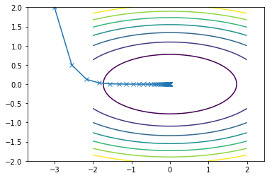
This is what the travel path of the SDM looks like for the two functions:

First function converges in 25 iterations

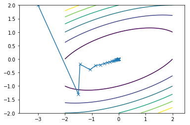
Second function converges in 36 iterations

Conjugate Direction methods

The main idea here is that the search direction is determined using conjugate vectors. These methods are more efficient in computing the search direction per iteration \(\approx\) \(O(n)\) whereas in Quasi-Newton methods the work per iteration is \(\approx$\)O(n^2)$$.

However, quality of the search direction \(p_k\) computed in these mehtods is lower than that of Quasi-Newton in the sense that convergence rate is slower. But the use case is dominated by the cheaper search computations for large \(n\).

What is conjugacy? \(\rightarrow\) Given a symmetric matrix Q, two vectors \(p_1\) and \(p_2\) are said to be Q-conjugate w.r.t Q if \(p_1^TQp_2 = 0\). If Q=I, conjugacy is the same as orthogonality as \(p_1^Tp_2 = 0\).

Why is conjugacy of interest \(\rightarrow\) Example: Consider the following (more general) quadratic optimization problem:

\[Min \ f(x) = \frac{1}{2}x^TQx-b^Tx\]

where Q is a nxn symmetric p.d matrix. Given a Q-orthogonal set \(\{p_i\}_{i=1}^n\) we can represent a point y as a linear combination of the n vectors in the Q-orthogonal set, i.e \(y = \sum_{i=1}^n \alpha_ip_i\). Evaluating \(f(y)\) we get:

\[\sum_{i=1}^n (\frac{1}{2} \alpha_i^2 p_i^T A p_i - \alpha_i b^T p_i)\]

Therefore, we reduce our orignial problem into $n$ one-dimensional sub-problems. Each of these one-dimensional problems can be solved by setting the derivative with respect to \(\alpha_i\) equal to zero:

\[\underset{y}{Min} \ f(y) = \sum_{i=1}^n \ \underset{\alpha_i}{Min} (\frac{1}{2} \alpha_i^2 p_i^T A p_i - \alpha_i b^T p_i) \\ where \ \alpha_i = \frac{b^Tp_i}{p_i^TAp_i}\]

Therefore, if we can represent the solution as a linear combination of conjugate vectors, then we can easily compute the \(\alpha_i\)’s and get the optimial solution \(x^* = \sum_{i=1}^n\frac{b^Tp_i}{p_i^TAp_i}p_i\).

What about other more general cases \(\rightarrow\) If Q is p.d and we have a set of non zero Q-orthogonal vectors then these vectors are linearly independent. This can be proved by contradiction.

If Q is p.d., then a Q-orthogonal set, comprised of n non zero vectors, forms a basis for $R^n$. i.e In other words, any point in \(x \in R^n\) can be represented as a linear combination of the \(n\) vectors in the Q-orthogonal set \(\{p_i\}_{i=1}^n\). This means that \(\forall x^*\in R^n\), we can always find \(\alpha_i\)’s such that: \(x^* = \sum_{i=1}^n\alpha_ip_i\).

Conjugate Direction Theorem: Let \(\{p_i\}_{i=1}^n\) be a set of non zero Q-orthogonal vectors. For any \(x_0 \in R^n\), the sequence \(\{x_k\}\) generated according to line search, \(x_{k+1} = x_k + \alpha_k p_k\) where \(\alpha_k = \frac{-\nabla f(x_k)_k^Tp_k}{p_k^TQp_k}\) converges to the unique solution, \(x^*\), of \(Qx = b\) after n steps, i.e \(x_n = x^*\).

So in Conjugate Direction Methods we assume that we have a Q-orthogonal set available to us. Whereas, in Conjugate Gradient Methods, the directions are not specified before hand, but are rather determined sequentially at each step of the iteration.

There many ways to compute this direction “\(p_i\)”, one way to that is:

\[p_0 = -\nabla f(x_0) \\ p_{k+1} = -\nabla f(x_{k+1}) + \beta_k p_k \\ where \ \beta_k = \frac{\nabla f(x_{k+1})^TQp_k}{p_k^TQp_k}\]

Algorithm:

Step 1: Given \(f(x)\), \(x_0\), set \(p_0 = -\nabla f(x_0)\)

Step2: While \(||\nabla f(x_k)|| > \epsilon\) \(\forall \ k \in {0,1,2...n}\)

(i) \(x_{k+1}= x_k + \alpha_k * p_k\), where \(\alpha_k\) is computed via line search

(ii) Calculate \(p_{k+1} = -\nabla f(x_{k+1}) + \beta_kp_k\) where \(\beta_k = \frac{-\nabla f(x_{k+1})^TQp_k}{p_k^TQp_k}\)

Implementation:

#### Conjugate Gradient Method
def CGM(sympy_function, max_iter, start, step_size, epsilon = 10**-2):
    i = 0
    x_values = np.zeros((max_iter+1,2))
    x_values[0] = start
    grad_fx = np.zeros((max_iter+1,2))
    p = np.zeros((max_iter+1,2))
    norm_values = []
    while i < max_iter:
        grad_fx[i] = df_x(sympy_function, x_values[i])
        norm = LA.norm(df_x(sympy_function, x_values[i]))
        if norm < epsilon:
            break
        else:
            if i == 0:
                beta = 0
                p[i] = - np.dot(step_size,df_x(sympy_function, x_values[i]))
            else:
                beta = np.dot(grad_fx[i],grad_fx[i]) / np.dot(grad_fx[i-1],grad_fx[i-1])
                p[i] =  -df_x(sympy_function, x_values[i]) + beta * p[i-1]
        x_values[i+1] = x_values[i] + step_size*p[i]
        norm_values.append(norm)
        i += 1
    print('No. of steps CDM takes to converge: ', len(norm_values))
    return(x_values, norm_values)

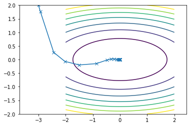
This is what the travel path of the CGM looks like for the two functions:

First function converges in 15 iterations

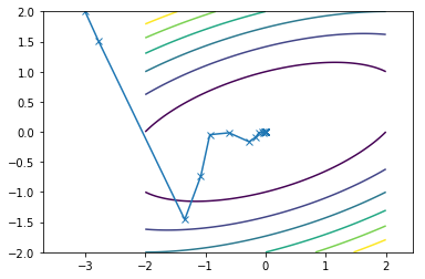
Second function converges in 14 iterations

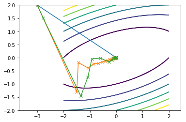
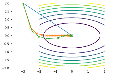
Here is what all of them combined look on the same contour plot where Newton is blue, SDM is orange and CGM is green:

First function:

Second function:

Code displayed in this post can be found on my github here.

References

Griva, I., & Nash, S. G. (2009). Linear and Nonlinear optimization. Philadelphia, PA: Society for Industrial and Applied Mathematics.