Maximum Clique Problem: Linear Programming Approach

12 minute read

Maximum Clique Problem was one of the 21 original NP-hard problems enumerated by Richard Karp in 1972. This post models it using a Linear Programming approach. In particular, we reduce the clique problem to an Independent set problem and solve it by appying linear relaxation and column generation.

Background

The clique problem arises in many real world settings. Most commonly in social networks which can be represented as a graph where the Vertices represent people and the graph’s edges represent connections. Then a clique represents a subset of people who are all connected to each other. So by using clique related algorithms we can find more information regarding the connections. Along with this, the clique problem also has many applications in computer vision and pattern recognition, patterns in telecommunications traffic, bioinformatics and computational chemistry.

An undirected graph has vertices that are connected together by undirected edges which we’ll represent as \(G = (V, E)\) where \(V = {1,2, . . , n}\) and \(E \subseteq V \times V\). A clique is a subset of vertices \(C \subseteq V\) in a graph such that there is an edge between any two vertices in the clique, \(i,j \in E\) for any \(i,j \in C\). An independent set is a subset of vertices \(C \subseteq V\) in a graph such that there is no edge between any two vertices in the independent set, \(i,j \notin E\) for any \(i,j \in C\).

A clique (independent set) is called maximal if it is not a subset of a larger clique (independent set) in \(G\), and maximum if there is no larger clique (independent set) in \(G\). The cardinality of a of a maximum clique in \(G\) is denoted \(\omega(G)\) and is called the clique number of \(G\). It is also known as the fractional clique number.

Visually:

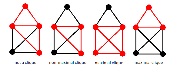
my alt text — image from: https://math.stackexchange.com/questions/758263/whats-maximal-clique

Given a graph \(G\) in which we want to find a clique, we can find a complement graph \(G'\) of \(G\) such that for every edge \(E\) in \(G\) there is no edge in \(G'\) and for every edge \(E\) that is not in \(G\) there is an edge in \(G'\). Now, if we find an independent set in \(G'\) it will be a clique in \(G\).

Modelling

Let \(I^*\) denote the set of all maximal independent sets in \(G\). Then the maximum clique problem can be formulated as the following integer program:

\[\begin{aligned} maximize & \; \sum_{j \in V} x_j\\ subject\;to\; & \sum_{j \in V} x_j \leq 1, \forall I \in I^*\\ & x_j \in \{0,1\}, \; j \in V. \end{aligned}\]

In the above equation the decision variable \(x_j \forall j \in V\) takes a biniary value. 1 if it is included in the maximum clique, 0 otherwise. The constraint of the above LP is has an upper bound of 1 as every maximal independent set can atmost have one vertex member of the set belonging to the maximum clique if there are more than 1 vertex in a maximal clique then that set is not independent. Moreover, note that constraint corresponds to every maximal independent set \(I \in I^*\). We now relax the model by replacing the integer constraints with non-negativity. We obtain the following linear program yielding an upper bound \(\bar{\omega} \geq \omega(G)\):

\[\begin{aligned} \bar{\omega}(G) = max & \sum_{j \in V} x_j\\ s.t. \; & \sum_{j \in V} x_j \leq 1,\;\; I \in I'\\ & x_j \geq 0, \; j \in V. \end{aligned}\]

To aid in column generation scheme we will formulate the dual of the above equation.

\[\begin{aligned} \bar{\omega}(G) = min & \sum_{I \in I^*} y_{I}\\ s.t. \; & \sum_{I \in I_j} y_{I} \geq 1,\;\; \forall j \in V\\ \end{aligned}\]

where \(I_j\) denote the set of all maximal independent sets containing vertex \(j \in V\).

Note that, for every linear programming problem there is a companion problem i.e “dual” linear program, in which the roles of variables and constraints are reversed.

In the above formulation, each variable represents a maximal independent set. Since generating the number of maximal independent sets in a graph is a NP-Hard problem as it is the same as finding the maximum clique in a compliment graph. We will use a greedy approach to generate a set of few maximal independent sets such that they cover all the vertices. The generated set \(I^\prime \subseteq I^*\) will used as the basis (column-wise) to initialize the restricted master problem (RMP). Below is the RMP:

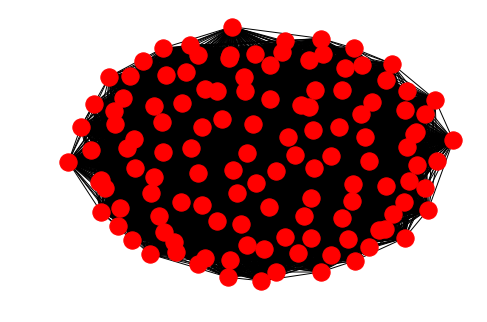
\[\begin{aligned} \bar{\omega}(G) = min & \sum_{I \in I^*} y_{I}\\ s.t. \; & \sum_{I \in I^\prime_j} y_{I} \geq 1,\;\; \forall j \in V\\ \end{aligned}\]

We would be implementing this post on a graph I obtained from my department. In order for it’s implementation first we will build a function to read the .txt file and convert it into a list where each vertex represents another list.

def preprocess(file):
  '''takes in the name of the file as a string and returns a list of edges'''
    f = open(file, 'r')
    lines = f.read().split("\n")
    col = [line.split() for line in lines] #split each line into a list
    condition = 'e' #all edges start with e
    wanted_list_3 = [i for i in col if(len(i) == 3)] #by len as some line may be empty
    wanted_list_e = [j for j in wanted_list_3 if(j[0] == condition)] #filter based on e
    wanted_list_s = [l[1:] for l in wanted_list_e] #only keep the edges
    wanted_list = [list(map(int, i)) for i in wanted_list_s] #convert string to int
    return (wanted_list)

In order to create the list of edges as a graph we use the networkx package in python. Traditionally we can use linked lists to represent the graph either as an adjacency list or an adjacency matrix. However, for this implementation we would use the networkx package which implements an adjacency list in the background.

def create_graph(edge_list):
    '''Takes in the list of edges as input and returns a graph'''
    elist = [tuple(x) for x in edge_list] #convert sub elements to tuple as req by networkx
    G = nx.Graph()
    G.add_edges_from(elist)
    print(G.number_of_nodes())
    return (G)

This is how our graph looks:

Now we create a greedy algorithm to find a good starting basis for the RMP by generating a subset \(I^\prime\) of maximal independent sets. We need to make sure that all the vertices of \(G\) are included in our subset in order to serve as a good starting basis.

#Main greedy algorithm
'''Takes in the graph and returns maximal independent sets'''
def greedy_init(G):
    n = G.number_of_nodes()                 #Storing total number of nodes in 'n'
    max_ind_sets = []                       #initializing a list that will store maximum independent sets
    for j in range(1, n+1):
        R = G.copy()                        #Storing a copy of the graph as a residual
        neigh = [n for n in R.neighbors(j)] #Catch all the neighbours of j
        R.remove_node(j)                    #removing the node we start from
        max_ind_sets.append([j])
        R.remove_nodes_from(neigh)          #Removing the neighbours of j
        if R.number_of_nodes() != 0:
            x = get_min_degree_vertex(R)
        while R.number_of_nodes() != 0:
            neigh2 = [m for m in R.neighbors(x)]
            R.remove_node(x)
            max_ind_sets[j-1].append(x)
            R.remove_nodes_from(neigh2)
            if R.number_of_nodes() != 0:
                x = get_min_degree_vertex(R)
    return(max_ind_sets)

where the get_min_degree_vertex subroutine is as follows:

def get_min_degree_vertex(Residual_graph):
  '''Takes in the residual graph R and returns the node with the lowest degree'''
    degrees = [val for (node, val) in Residual_graph.degree()]
    node = [node for (node, val) in Residual_graph.degree()]
    node_degree = dict(zip(node, degrees))
    return (min(node_degree, key = node_degree.get))

The algorithm works as follows. For each vertex \(j\), starting with \(j\), all neighbours of \(j\) are removed, and then, at each step, a minimum degree vertex is chosen from the residual graph \(R\) and added to the maximal independent set of vertex \(j\). Subsequently, as vertices are added to the set, their neighbours are removed and the steps are repeated until the residual graph is empty. This algorithm thus leaves us with a set of maximal independent sets for each \(j \in V\).

Now let us implement the RMP model in Gurobi:

#GUROBI
#RMP MODEL
y_var = {}
temp = {}
#Create a set I' for obj function summation
set_I = range(1, n+1) #n = no. of nodes in graph G

#Create a set for constraint summation
set_II = max_ind_sets #max_ind_sets are the maximal independent sets obtained from our greedy algorithm
#Define an optimization model
rmp_model = grb.Model(name="RMP")
rmp_model.setParam(grb.GRB.Param.Presolve, 0)
rmp_model.setParam('OutputFlag', False) #To deactivate unneccessary output
#Create a continous decision variable 'y'
for i in set_I:
    y_var[i] = rmp_model.addVar(obj=1, lb=0.0, vtype=grb.GRB.CONTINUOUS, name="y_var[%d]"%i)
#Create constraints
# >= constraints
x = 0
for i in set_II:
    x = x+1
    var = [y_var[k] for k in i]
    coef = [1] * len(i)
    temp[x] = rmp_model.addConstr(grb.LinExpr(coef,var), ">", 1, name="temp[%d]"%x)
#Objective Function
objective = grb.quicksum(y_var[j]
                         for j in set_I)
rmp_model.setObjective(objective, grb.GRB.MINIMIZE)
rmp_model.write('rmp_day2.lp') #Write model to an LP file to verify

Now we use the decomposition principle to transform the RMP into a Column generation subproblem (CGSP) which is:

\[\begin{aligned} w = \underset{I \in I^*} max \sum_{j \in I} (d_j -1) \\ \end{aligned}\]

where \(d\) represent the dual prices of the RMP. Therefore, the CGSP is a maximum weight independent set problem seeking to find an independent set maximizing the sum of vertex weights in \(G\), where the weights are given by the dual \(d\).

The CGSP can be solved using the following IP formulation which we will feed into our CGSP gurobi model.

\[\begin{aligned} max & \sum_{j \in V} d_jx_j\\ s.t. \; & x_i + x_j \leq 1,\;\; \{i, j\} \in E \\ & x_j \in \{0,1\} \; j \in V. \end{aligned}\]

#CGSP

#set of vertices
set_III = edge_list
#Define an optimization model
cgsp_model = grb.Model(name = "CGSP")
cgsp_model.setParam(grb.GRB.Param.Presolve, 0)
cgsp_model.setParam('OutputFlag', False)
#Create a biniary decision variable
x_var = {}
for j in set_I:
    x_var[j] = cgsp_model.addVar(obj = 1, vtype = grb.GRB.BINARY, name = "x_var[%d]"%j)
#create constraints
temp2 = {}
y = 0
for (i,j) in set_III:
    y = y+1
    var1 = [x_var[i]]
    coef1 = [1]
    var2 = [x_var[j]]
    coef2 = [1]
    expr = grb.LinExpr(coef1, var1)
    expr.addTerms(coef2, var2)
    temp2[y] = cgsp_model.addConstr(expr, grb.GRB.LESS_EQUAL, 1, "temp2[%d]"%y)
cgsp_model.write('day2_cgsp.lp')

We create another function to update our CGSP objective based on the dual values obtained each iteration from solving the RMP.

def update_obj(dual):
    var3 = [x_var[j] for j in set_I]
    coef3 = [dual[j-1] for j in set_I]
    objective2 = grb.LinExpr(coef3, var3)
    cgsp_model.setObjective(objective2, grb.GRB.MAXIMIZE)
    cgsp_model.update()
    ob = cgsp_model.getObjective()
    #print(ob)
    cgsp_model.write('cgsp.lp')

Now we run our model in a loop with a termination condition.

#Column generation
K = len(set_I) + 1

while True:
    rmp_model.optimize()                        #solve the RMP
    print('RMP_Objective : ', rmp_model.ObjVal)
    dual = get_dual(rmp_model)                  #get dual from the 'rmp_model'
    update_obj(dual)                            #update CGSP objective
    cgsp_model.optimize()                       #solve the CGSP
    x_values = cgsp_model.x
    print('CGSP_Objective : ', cgsp_model.ObjVal)
    if cgsp_model.ObjVal <=1.001:
        break
    else:
        col = grb.Column()
        for i in range(1,n):
            col.addTerms(x_values[i-1], temp[i]) #add column to RMP
        y_var[K] = rmp_model.addVar(obj=1, vtype=grb.GRB.CONTINUOUS, name="y_var[%d]"%K, column = col)
        rmp_model.update()
        rmp_model.write('updated.lp')
        K += 1

Below is the output for the input graph.

RMP_Objective : 45.0

CGSP_Objective : 2.0

RMP_Objective : 45.0

CGSP_Objective : 2.0

RMP_Objective : 45.0

CGSP_Objective : 2.0

RMP_Objective : 45.0

CGSP_Objective : 2.0

RMP_Objective : 45.0

CGSP_Objective : 2.0

RMP_Objective : 45.0

CGSP_Objective : 2.0

RMP_Objective : 44.5

CGSP_Objective : 2.0

RMP_Objective : 44.0

CGSP_Objective : 2.0

RMP_Objective : 44.0

CGSP_Objective : 2.0

RMP_Objective : 44.0

CGSP_Objective : 2.0

RMP_Objective : 44.0

CGSP_Objective : 2.0

RMP_Objective : 44.0

CGSP_Objective : 2.0

RMP_Objective : 44.0

CGSP_Objective : 2.0

RMP_Objective : 44.0

CGSP_Objective : 2.0

RMP_Objective : 44.0

CGSP_Objective : 2.0

RMP_Objective : 44.0

CGSP_Objective : 2.0

RMP_Objective : 44.0

CGSP_Objective : 2.0

RMP_Objective : 44.0

CGSP_Objective : 2.0

RMP_Objective : 44.0

CGSP_Objective : 2.0

RMP_Objective : 44.0

CGSP_Objective : 2.0

RMP_Objective : 44.0

CGSP_Objective : 2.0

RMP_Objective : 44.0

CGSP_Objective : 2.0

RMP_Objective : 44.0

CGSP_Objective : 2.0

RMP_Objective : 44.0

CGSP_Objective : 2.0

RMP_Objective : 44.0

CGSP_Objective : 2.0

RMP_Objective : 44.0

CGSP_Objective : 2.0

RMP_Objective : 44.0

CGSP_Objective : 2.0

RMP_Objective : 44.0

CGSP_Objective : 2.0

RMP_Objective : 44.0

CGSP_Objective : 2.0

RMP_Objective : 44.0

CGSP_Objective : 2.0

RMP_Objective : 44.0

CGSP_Objective : 2.0

RMP_Objective : 44.0

CGSP_Objective : 2.0

RMP_Objective : 44.0

CGSP_Objective : 2.0

RMP_Objective : 44.0

CGSP_Objective : 2.0

RMP_Objective : 44.0

CGSP_Objective : 2.0

RMP_Objective : 44.0

CGSP_Objective : 2.0

RMP_Objective : 44.0

CGSP_Objective : 2.0

RMP_Objective : 44.0

CGSP_Objective : 2.0

RMP_Objective : 44.0

CGSP_Objective : 2.0

RMP_Objective : 43.0

CGSP_Objective : 2.0

RMP_Objective : 43.0

CGSP_Objective : 2.0

RMP_Objective : 43.0

CGSP_Objective : 2.0

RMP_Objective : 43.0

CGSP_Objective : 2.0

RMP_Objective : 43.0

CGSP_Objective : 2.0

RMP_Objective : 43.0

CGSP_Objective : 2.0

RMP_Objective : 43.0

CGSP_Objective : 2.0

RMP_Objective : 43.0

CGSP_Objective : 2.0

RMP_Objective : 43.0

CGSP_Objective : 2.0

RMP_Objective : 43.0

CGSP_Objective : 2.0

RMP_Objective : 43.0

CGSP_Objective : 2.0

RMP_Objective : 43.0

CGSP_Objective : 2.0

RMP_Objective : 43.0

CGSP_Objective : 2.0

RMP_Objective : 42.5

CGSP_Objective : 2.0

RMP_Objective : 42.5

CGSP_Objective : 2.0

RMP_Objective : 42.5

CGSP_Objective : 1.5

RMP_Objective : 42.5

CGSP_Objective : 1.5

RMP_Objective : 42.5

CGSP_Objective : 1.5

RMP_Objective : 42.5

CGSP_Objective : 1.5

RMP_Objective : 42.5

CGSP_Objective : 1.5

RMP_Objective : 42.5

CGSP_Objective : 1.5

RMP_Objective : 42.5

CGSP_Objective : 1.5

RMP_Objective : 42.5

CGSP_Objective : 1.5

RMP_Objective : 42.5

CGSP_Objective : 1.6666666666666665

RMP_Objective : 42.5

CGSP_Objective : 1.5

RMP_Objective : 42.5

CGSP_Objective : 1.5

RMP_Objective : 42.5

CGSP_Objective : 1.5

RMP_Objective : 42.5

CGSP_Objective : 1.5

RMP_Objective : 42.5

CGSP_Objective : 1.5

RMP_Objective : 42.5

CGSP_Objective : 2.0

RMP_Objective : 42.5

CGSP_Objective : 2.0

RMP_Objective : 42.25

CGSP_Objective : 2.0

RMP_Objective : 42.099999999999994

CGSP_Objective : 1.8

RMP_Objective : 42.0

CGSP_Objective : 2.0

RMP_Objective : 41.875

CGSP_Objective : 1.75

RMP_Objective : 41.625

CGSP_Objective : 1.75

RMP_Objective : 41.625

CGSP_Objective : 1.7499999999999993

RMP_Objective : 41.625

CGSP_Objective : 1.7499999999999971

RMP_Objective : 41.5

CGSP_Objective : 2.0

RMP_Objective : 41.5

CGSP_Objective : 1.5

RMP_Objective : 41.5

CGSP_Objective : 1.5

RMP_Objective : 41.5

CGSP_Objective : 1.5

RMP_Objective : 41.0

CGSP_Objective : 1.5

RMP_Objective : 41.0

CGSP_Objective : 1.5

RMP_Objective : 41.0

CGSP_Objective : 1.4761904761904763

RMP_Objective : 41.0

CGSP_Objective : 1.4705882352941178

References

Griva, I., & Nash, S. G. (2009). Linear and nonlinear optimization. Philadelphia, PA: Society for Industrial and Applied Mathematics.