
Ranking teams using Discrete Time Markov Chains
Ranking methods are an essential tool in making decisions. They have many applications from sports to web searches to recommender systems. One of the most popular ranking algorithm is Google’s Page Rank algorithm that also uses the notion of Markov Chains in some capacity. In this post we use Discrete Time Markov Chains (DTMC’s) to rank 32 NFL teams after the regular season.
Introduction
The National Football League (NFL) is a professional American football league consisting of 32 teams, divided equally between the National Football Conference (NFC) and the American Football Conference (AFC). Both conferences consist of four four-team divisions. Each team plays 16 regular-season games; thus, teams do not play all other teams during a single regular season. We will be using scores from the 2007 regular season, can be downloaded from: link.
Modelling
Naturally, we will consider each team to correspond to each state in the Markov chain.
Therefore, Our state space will be the total no. of football teams in NFL represented as \(X_n \forall n \in {0,1,2...31}\).
We introduce a new paramter \(F\) i.e Football fans where \(f\) is an individual fan.
Initially, we assume that football fans are equally distributed among all the teams i.e \(F_0 = F_1 = F_2 = ... = F_{31}\)
Then,
\(\exists\) \(P_{i,j}\) \(\forall\) \(i = j\) i.e Transition exists for all the teams that have played each other
\(\nexists\) \(P_{i,j}\) \(\forall\) \(i \ne j\) i.e Transition does not exist for all the teams that have not played each other
Based on the values of scores (subjective to the approach used), we assume that after each match a fan makes a decision to move i.e switch allegiance from one team to another. Eventually, we consider the team with the highest no. of fans to be ranked 1.
Note that, movement of fans here is an arbitirary concept and it is the same as saying chances of winning the Vince Lombardi Trophy, \(t\), where after each match \(t\) moves from team \(i \longrightarrow j\) or \(j \longrightarrow i\). So, in conclusion here we are simply equating \(F\) (No. of fans) to chances of winning the trophy.
With this construct we can say that our problem is a first order Markov Chain as
\(P(X_{n+1} = j| X_n = i )\) and \(P(X_{n+1} = i| X_n = j)\).
Approach 1 : Using both PtsW and PtsL
In the first approach we will be utilising the points won (PtsW) and points lost (PtsL) by each team.
data = pd.read_csv('data_2007.csv') #reading in the file
data = data.rename(index = str, columns = {"Winner/tie": "Winner", "Loser/tie": "Loser"})
data.Winner.isnull() #256 to 267 rows are null i.e Playoff rows
data = data[0:256]
list(data.columns) #names of all the columns
In this approach at each iteration,
\[f_{i,k} \longrightarrow f_{j,k+1}\]- A fan moves from losing team to winning team based on PtsW i.e points scored by the winning team
- A fan moves from the winning team to losing team based on PtsL i.e points scored by the losing team
Note that, in this case a fan does not move from the same team to itself i.e \(f_{i,k} \not\to f_{i,k+1}\) as we are explicitly using scores and there is naturally no PtsW and PtsL data for a team against itself. Therefore, by extension: \(\nexists P_{i,i} \forall i\)
Now, we will show that our Markov chain is irreducible and aperiodic. This is to utilize an essential property of Markov chains which is:
\[\begin{aligned} \lim_{n \to \infty} p^n_{i,j} = \pi_j, \forall i,j \in S \\ \end{aligned}\]For an irreducible positive recurrent DTMC, there exist \({\pi_j > 0, j \in S}\) such that
where the \(\pi_j\) is the unique solution to:
\[\begin{aligned} \pi_j = \sum_{i \in S} \pi_i p_{i,j}, \forall j \in S \\ \sum_{j \in S} = 1 \end{aligned}\]Note that, for finite states an irreducible and aperiodic DTMC is positive reccurent.
On an intutive level: if a DTMC is positive recurrent and we take it’s probability transition matrix to infinity then it’s transition probability values of moving from one state to another will converge to a steady state distribution.
Proving it is irreducible.
Our Markov Chain is irreducible simply by how the league is scheduled. To elaborate, in an NFL league each team plays 16 games each season.
- Twice agianst each team in their division (6)
- 4 games against a division in the other league (4)
- 4 games against another division in their league (4)
- 1 game each against two of the remaining divisions in their league (2)
So a team is connected to all the other 32 teams.
Proving aperiodicity.
For aperiodicity, first consider one division where all 4 teams play each other twice. We will have 4 bi-directed states that are all connected to each other. Note that a Markov chain is aperiodic if there are 3 or more fully connected bidirected states. By extension, our division is aperiodic. Now as our chain is irreducible and since aperiodicity is a class property, our entire model is also aperiodic.
Now, that we have proved that our markov chain is irreducible and aperiodic we can use above mentioned property of \(\pi = \pi P\) to obtain the steady state vector \(\pi\) which can then be used to rank the teams.
Below is the code to generate a transition matrix from the csv file downloaded.
df2 = pd.DataFrame(np.random.randint(low=0, high=1, size=(32, 32)), columns=['Arizona Cardinals', 'Atlanta Falcons', 'Baltimore Ravens',
       'Buffalo Bills', 'Carolina Panthers', 'Chicago Bears',
       'Cincinnati Bengals', 'Cleveland Browns', 'Dallas Cowboys',
       'Denver Broncos', 'Detroit Lions', 'Green Bay Packers',
       'Houston Texans', 'Indianapolis Colts', 'Jacksonville Jaguars',
       'Kansas City Chiefs', 'Miami Dolphins', 'Minnesota Vikings',
       'New England Patriots', 'New Orleans Saints', 'New York Giants',
       'New York Jets', 'Oakland Raiders', 'Philadelphia Eagles',
       'Pittsburgh Steelers', 'San Diego Chargers', 'San Francisco 49ers',
       'Seattle Seahawks', 'St. Louis Rams', 'Tampa Bay Buccaneers',
       'Tennessee Titans', 'Washington Redskins'])

my_dict = {'Arizona Cardinals' : 0, 'Atlanta Falcons' : 1, 'Baltimore Ravens' : 2,
       'Buffalo Bills' : 3, 'Carolina Panthers' : 4, 'Chicago Bears' : 5,
       'Cincinnati Bengals' : 6, 'Cleveland Browns' : 7, 'Dallas Cowboys' : 8,
       'Denver Broncos' : 9, 'Detroit Lions' : 10, 'Green Bay Packers' : 11,
       'Houston Texans' : 12, 'Indianapolis Colts' : 13, 'Jacksonville Jaguars' : 14,
       'Kansas City Chiefs' : 15, 'Miami Dolphins' : 16, 'Minnesota Vikings' : 17,
       'New England Patriots' : 18, 'New Orleans Saints' : 19, 'New York Giants' : 20,
       'New York Jets' : 21, 'Oakland Raiders' : 22, 'Philadelphia Eagles' : 23,
       'Pittsburgh Steelers' : 24, 'San Diego Chargers' : 25, 'San Francisco 49ers' : 26,
       'Seattle Seahawks' : 27, 'St. Louis Rams' : 28, 'Tampa Bay Buccaneers' : 29,
       'Tennessee Titans' : 30, 'Washington Redskins' : 31}


data2 = data[['Winner', 'Loser', 'PtsW', 'PtsL']]

############
#Function to assign Loser -> Winner scores (L -> W, PtsW)
def L_W(data, my_dict, winner, data2):
    for loser in data.loc[data.Winner == winner, 'Loser'].unique():
        for team, value in my_dict.items():
            if loser == team:
                i = value
                l = sum(data.loc[(data.Loser == loser) & (data.Winner == winner), 'PtsW'].values)
                j = winner
                data2.loc[i, j] = l
    return(data2)

t1 = data[['Winner', 'Loser', 'PtsW']]
win_team = t1.Winner.unique()
for winner in win_team:
    L_W(t1, my_dict, winner, df2)

#Function to assign Winner -> Loser score (W -> L, PtsL)

def W_L(data, my_dict, winner, data2):
    for loser in data.loc[data.Winner == winner, 'Loser'].unique():
        for team, value in my_dict.items():
            if winner == team:
                i = value
                l = sum(data.loc[(data.Loser == loser) & (data.Winner == winner), 'PtsL'].values)
                j = loser
                data2.loc[i, j] = l
    return(data2)

t2 = data[['Winner', 'Loser', 'PtsL']]
for winner in win_team:
    W_L(t2, my_dict, winner, df2)
This is what our transition matrix looks like:
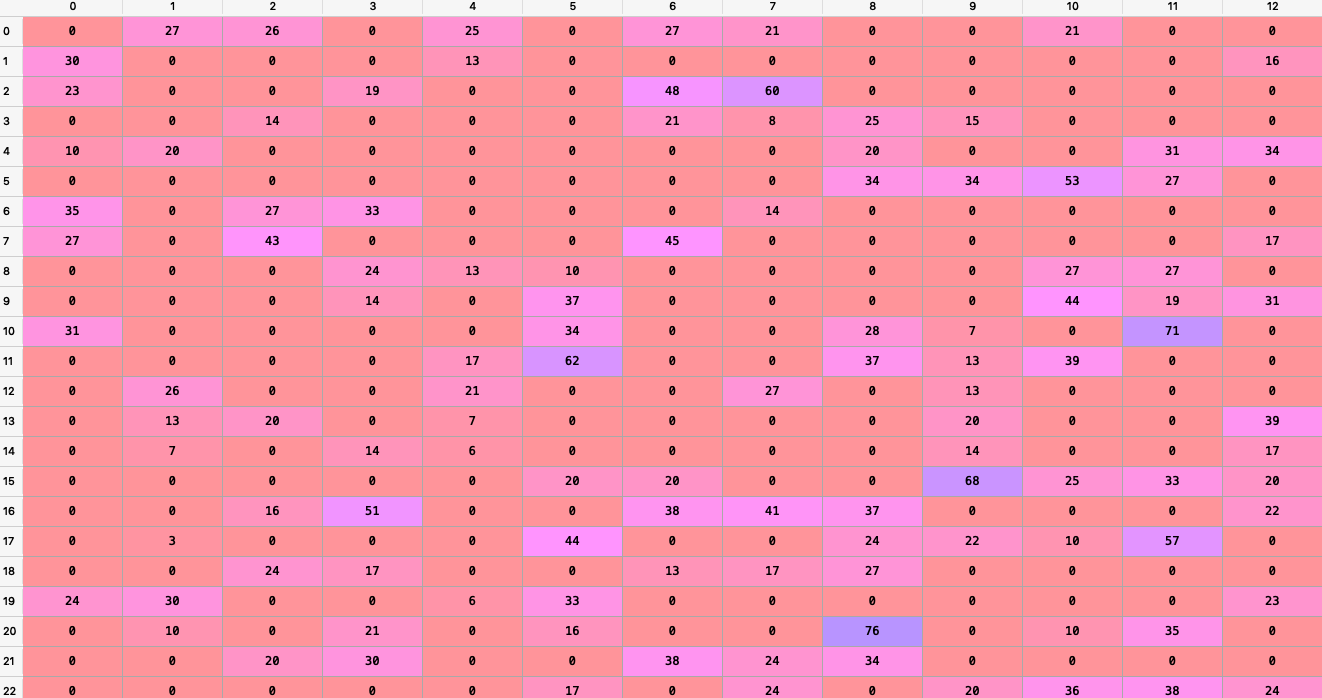
Note, that we need to normalize the values of the matrix such that all the rows add up to 1. We do this as the transition matrix should be a stochastic matrix.
#Sum by row
row_sum = df2.sum(axis = 1).to_dict()
transition_mat = df2.values


final_mat  = transition_mat/transition_mat.sum(axis = 1)[:, None]
final_mat.sum(axis = 1) #All rows add up to 1
Now, we raise the matrix to a high power to find it’s liming distribution.
raised_mat = matrix_power(final_mat, 10000)
Here is what it looks like after converging:
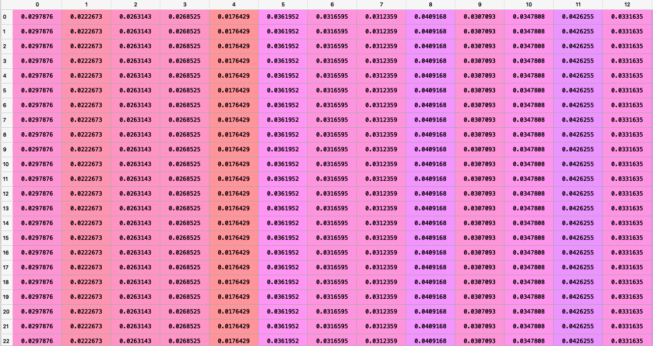
Note that:
- In cases where there were two matches between teams we have taken the sum of Ptsw and PtsL.
- The images only display a partial matrix.
After ranking the steady state \(\pi\) vector this is what we get:
steady_state = dict(enumerate(raised_mat[1]))
#Sort dictionary by value
rank = sorted(steady_state, key = steady_state.get, reverse = True)

#Result
for r in rank:
    for name, state in my_dict.items():
        if r == state:
            print(name)
- New England Patriots
- Indianapolis Colts
- Green Bay Packers
- Dallas Cowboys
- San Diego Chargers
- New York Giants
- Chicago Bears
- Detroit Lions
- Jacksonville Jaguars
- Minnesota Vikings
- Houston Texans
- Philadelphia Eagles
- New Orleans Saints
- Cincinnati Bengals
- Cleveland Browns
- Pittsburgh Steelers
- Denver Broncos
- Arizona Cardinals
- Miami Dolphins
- Washington Redskins
- New York Jets
- Seattle Seahawks
- Buffalo Bills
- Tampa Bay Buccaneers
- Baltimore Ravens
- Tennessee Titans
- Oakland Raiders
- St. Louis Rams
- Atlanta Falcons
- Kansas City Chiefs
- San Francisco 49ers
- Carolina Panthers
Approach 2 : Using absolute wins and losses
The same construct that we defined in the Approach 1 carries over to this one with the only difference being that instead of PtsW and PtsL we consider wins and losses of a team.
At each iteration,
\[f_{i,k} \longrightarrow f_{j,k+1}\]- A fan moves from the losing team to the winning team with a probability \(p \in (0.5, 1)\)
- A fan moves from the winning team to losing team with probability \(1-p\)
Note that, the probability of a fan moving to a winning team should be higher than a losing team. Mathamatically, \(P(f_{i_w})>P(f_{j_l})\)
Secondly, if two teams have equal wins and loses against each other then the transitions between the two teams are considered to be equally likely in either direction i.e \(f_{i,j} = f_{j,i} = 0.5\).
The chain is irreducible and aperiodic due to the same reasons as mentioned in Approach 1.
In this case we choose an arbitirary p value of \(0.8\)
#Function to create a transition matrix
p = 0.8 #arbitrary value selected
q = 0.2 #arbitrary value selected
def get_matrix(data_original, team, data_state, team_dict):
    '''Takes in the original dataframe, team, empty transition matrix and dictionary to give
    a transition matrix based on values of p and 1'''
    t1 = data_original.loc[data_original.Winner == team, 'Loser'].unique() #Teams supplied 'team' WON against
    t2 = data_original.loc[data_original.Loser == team, 'Winner'].unique() #Teams suuplied 'team' LOST again
    t3 = np.intersect1d(t1,t2) #Teams supplied 'team' both won and lost against, p = 0.5 for this
    t1 = np.setdiff1d(t1,t3) #Removing the intersection for WON
    t2 = np.setdiff1d(t2,t3) #Removing the intersection for LOST
    for name, state in team_dict.items():
        if name == team:
            l = state #l is the state space number
    for i in t1:
        data_state.loc[l, i] = q
    for j in t2:
        data_state.loc[l, j] = p
    for k in t3:
        data_state.loc[l, k] = 0.5
    return(data_state)

for i in teams:
    get_matrix(data, i, df2, my_dict)
Using \(\pi = \pi P\) and ranking the steady state \(\pi\) vector this is what we get:
- New England Patriots
- Dallas Cowboys
- Green Bay Packers
- San Diego Chargers
- Indianapolis Colts
- Washington Redskins
- Jacksonville Jaguars
- Philadelphia Eagles
- New York Giants
- Chicago Bears
- Minnesota Vikings
- Tennessee Titans
- Denver Broncos
- Houston Texans
- Detroit Lions
- Cleveland Browns
- Pittsburgh Steelers
- Buffalo Bills
- Tampa Bay Buccaneers
- New Orleans Saints
- Seattle Seahawks
- Carolina Panthers
- Arizona Cardinals
- Cincinnati Bengals
- Kansas City Chiefs
- Baltimore Ravens
- New York Jets
- Oakland Raiders
- Atlanta Falcons
- Miami Dolphins
- San Francisco 49ers
- St. Louis Rams
All the code for this project can be found on my here.
References
- NFL league scheduling: https://www.youtube.com/watch?v=KGKwTnaV-rg
- Data from https://www.pro-football-reference.com/years/2007/games.html
- Background reading:
- “Discrete-Time Markov Chains: Limiting Behavior.” Introduction to Modeling and Analysis of Stochastic Systems, by Vidyadhar G. Kulkarni, Springer, 2011.
- Vaziri, B. (n.d.). Markov-based ranking methods
- Mattingly, R (n.d.). A Markov Method for Ranking College Football Conferences