Predictive maintenance: A time series approach

Unexpected downtime has a significant effect on throughput in manufacturing. Managing the service life of equipment helps in reducing downtime costs. The ability to predict equipment outage helps in deploying pre-failure maintenance and bring down unplanned downtime costs. Quite commonly, these machines produce streams of time series data which can be modeled using markovian techniques. In this post we look at using time series techniques to forecast the failure of such machines.   In particular we’ll be using ARIMA and a single layer perceptron model on the C-MAPSS dataset from NASA’s prognostics data repository, part of a challenge known as Prognostics and Health Management (PHM08). You can find the dataset here.

Introduction

First, let us look at the dataset characteristics:

Data is a from a fleet of 4 similar simulated aircraft engines operating under different conditions. Data is available from 21 internal sensors and 3 external sensors. This data is contaminated with sensor noise where in each case the engine is operating normally at the start of each time series and develops a fault at some point during the series and eventually deteriorates until failure. Each dataset is divided into:

1. Training: In the training set, the fault grows in magnitude until system failure.
2. Test: In the test set, the time series ends some time prior to system failure.
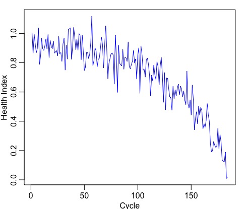
3. RUL vector: Delta of (actual failure - last sensor observation) from the test set. 4. Clearly, these datasets were geared towards data-driven approaches where very little or no system information was made available. The fundamental difference between these 4 datasets is attributed to the number of simultaneous fault modes and the operational conditions simulated in these experiments. In this post, we will be working with the first simulated dataset. Note that the first dataset has 100 different engines within it. Below is a visual interpretation of the dataset:

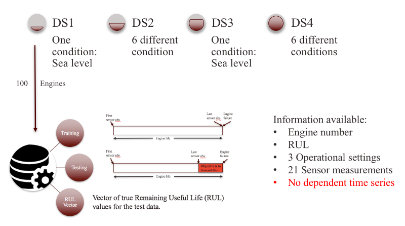
Our objective is to forecast the RUL of the test set i.e the red colored portion in the above image. 

Preprocessing:

1. Sensor selection:

Plots of 21 sensor measurements

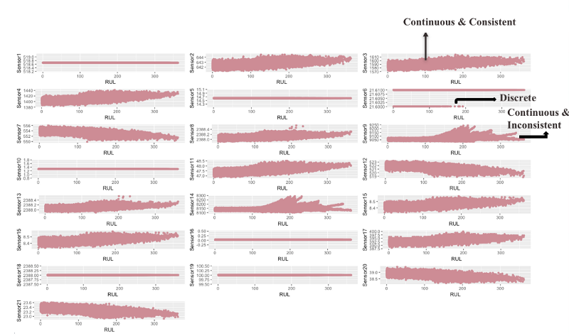
The scatter plots above give us an intuition regarding the health of the engine w.r.t to various sensors. However, not all sensors are equally important as some of them do not provide any information and others provide conflicting evidence. Therefore, based on the sensor patterns, we classify them into three categories: 1) Continuous and consistent 2) Discrete and 3) Continuous and Inconsistent.

Sensors that have one or more discrete values do not increase our understanding of the engine health hence can be eliminated. Sensors that have continuous but inconsistent values may contain some hidden information but due to inconsistencies towards the end they tend to be rather misleading and therefore need to be eliminated as well. Only sensors that have continuous and consistent values are chosen i.e (sensors 2, 3, 4, 7, 8,11, 12, 13, 15, 20 and 21). These sensors will aid in modelling a mathematical function to describe engine degradation.

Plots of the 3 operational settings

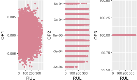
All three operational settings are ignored based on the sensor selection criteria. 

2. Health Index:

The intuition behind using a health index is to model a univariate time series, as a function of the selected sensors, that will help us understand the degradation pattern of each engine. 

In order to do so, first we would need a target variable w.r.t to which various sensor inputs can be modelled. As we do not have a target variable we will create one for each of the 100 engines, in the training set, by selecting the first 30 cycles and labelling them as 1 (assuming they represent a healthy condition) and the last 30 cycles as 0 (assuming they represent a deteriorated condition). 

You could probably ask why 30? 

So, first, we first look at the summary of max RUL

#Look at the RUL summary
RUL_engine = aggregate(RUL~Engine, data, max)
summary(RUL_engine$RUL)

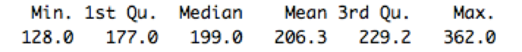
which gave us 128 as the minimum value. Now, in these 128 cycles naturally first few are good and the last few are bad as the engine starts well and then eventually deteriorates. To give us some breathing space and to clearly distinguish between good and bad we divide by 2 to attain 64. Now, in these 64 we can assign the first half as 1 and the last half as 0 but for better symmetry we choose 30. 

HI for engine 1 in the training set

After assigning 0’s /1’s, removing null values and keeping only the required sensors. We look at the correlation between the remaining sensors and the manually curated health index.

Correlation plot between continuous - consistent sensors and health index

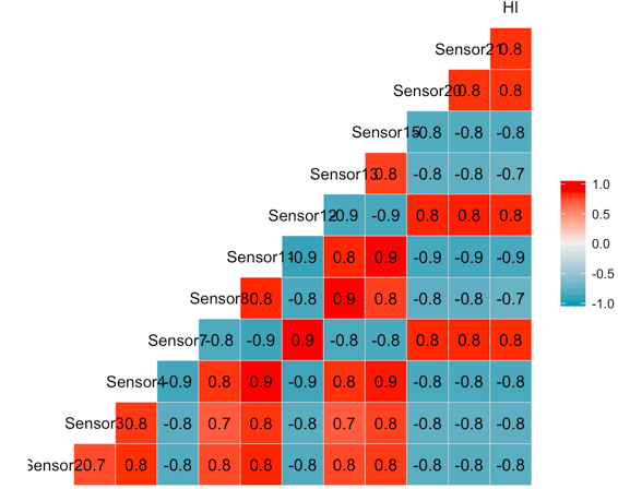
As we can observe from the above correlation plot, all the sensors have a significant correlation with the HI. Therefore, we will proceed without eliminating any of them.

Now, we will use our target i.e HI and features i.e continuous and consistent sensors, to create a model which will give us the HI on the test set. We will employ a linear regression to do so. 

\[\begin{aligned} Y = \beta_0 + \beta_1 x_1 + \beta_2 x_2 + \beta_3 x_3 + ... + \beta_k x_k + \epsilon \end{aligned}\]

The above regression equation gives us estimated parameters. Using these regression parameters on our test set, we will obtain an HI for all the 100 engines in the test set. The HI for each of those engine will be a univariate time series which can be modeled using Time series techniques.

#Using regression on the training set to obtain a health index
regression = lm(HI~., data = data_final)

This model stored in regression can now be used on the test set to create a univariate time series aka a health index that will help us understand the degradation pattern of each engine.

#reading in the test file
test = read.csv("test.csv")
test_s = subset(test, select = c("S2","S3","S4",
                                   "S7","S8","S11"
                                   ,"S12","S13","S15",
                                   "S20","S21"))
colnames(test_s) = c("Sensor2","Sensor3","Sensor4",
                      "Sensor7","Sensor8","Sensor11",
                      "Sensor12","Sensor13","Sensor15",
                      "Sensor20","Sensor21")
test_model = predict.lm(regression, test_s) #using the regression parameters to get HI
test_s$HI = test_model #Found HI
test = cbind(test, test_s$HI) #Cbind HI with original test

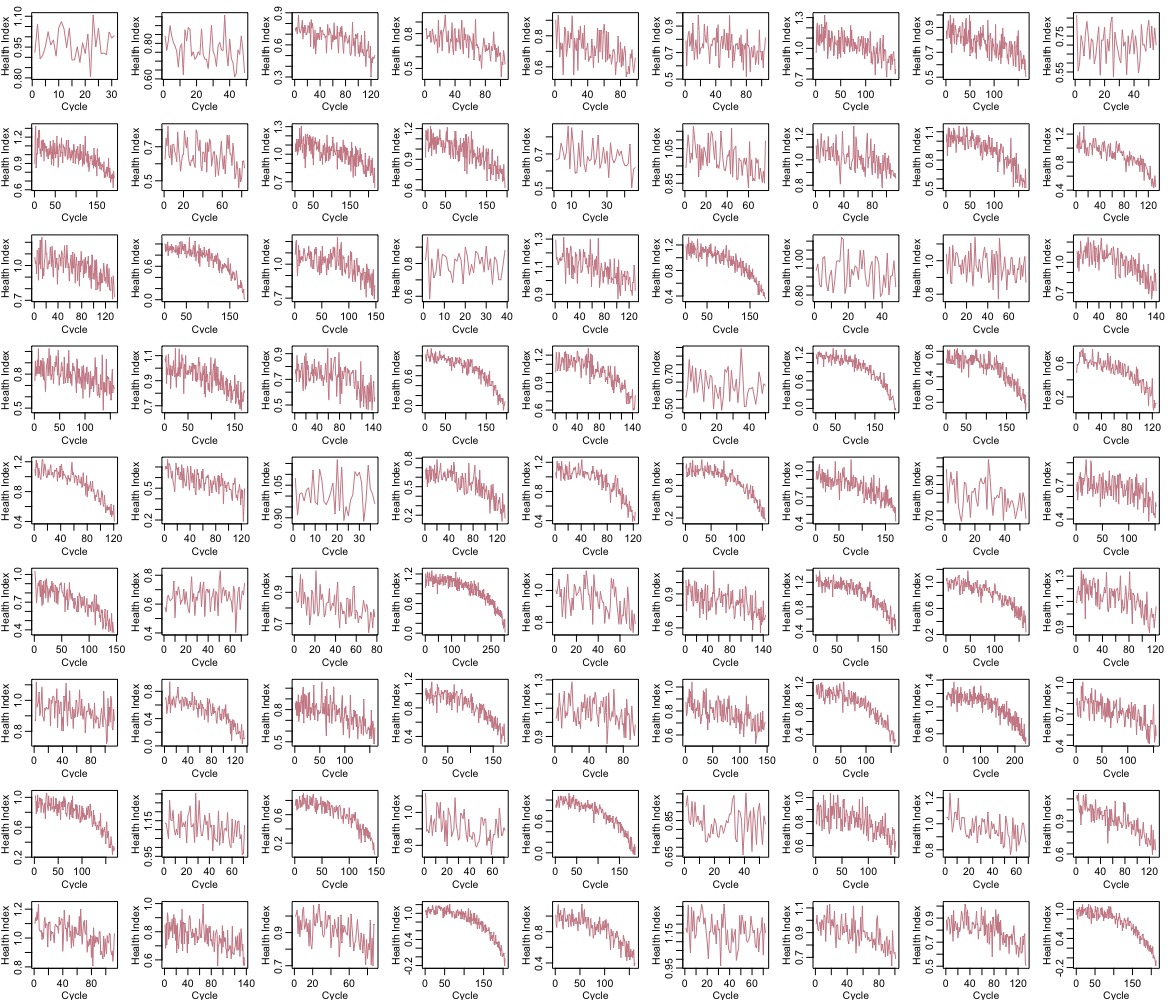
The below code will plot HI for all the 100 engines

#creating a function to map engine to the ts.plot function
plot_hi = function(j){
  test_1 = test[test$Engine == j,]
  case1 = test_1$`test_s$HI`
  ts.plot(case1, col = 'lightpink3', xlab = 'Cycle', ylab = 'Health Index')
}

engines = 1:100

hilist = list()
for (j in engines){
  hilist[[j]] = plot_hi(j)
}

Below is the HI for 81 of the 100 engines:

Health Index (HI) of 81 engines

Now, we will select 9 of these engines to forecast RUL. Below is the plot of the 9 engines selected:

Row 1 - Low RUL, Row 2 - Med RUL, Row 3 - High RUL

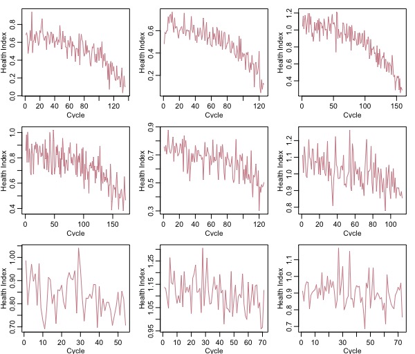
We have selected these engine’s such that 3 of them have a low RUL, 3 have medium RUL and 3 have a lot of useful life before failure. This is to see how effective our algorithm would be in a real world stochastic situation.

From the above image it appears as though the time series in the first two row’s have a stochastic trend while the last row looks almost stationary. This is important because based on if the series has a trend or not we would have to convert it to stationarity and supply it to our model. To test for stationarity let us perform the Kwiatkowski-Phillips-Schmidt-Shin (KPSS) test for the null hypothesis, \(H_0\) that our series is stationary.

#Performing kpss test to test stationarity
stationary_result = lapply(forecast_list2, kpss.test, null = "Level") #Level means that the data is like white noise
print(stationary_result)

Here null = “Level” argument test for the null hypothesis, \(H_0\) that our series is stationary. Naturally, if our p-value is less \(\alpha = 0.05\) we reject \(H_0\) and it means that our series has a trend and differencing would be required to make it stationary.

Below is the image of the p-value obtained after the KPSS test:

This marks the end of preprocessing.

Modelling

We’ll be using two modelling techniques as mentioned earlier.

ARIMA

ARIMA is a classic statistical approach to model univariate data. An ideal approach in using ARIMA(p,d,q) is to:

1. Plot the time series to check if it is stationary:

1. If the series is not stationary, make it by differencing (to remove trend) or apply a power transformation (to stablize variance): -> this is the d part.

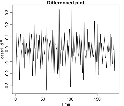
1. Plot the ACF/PACF of the stationary series to identify AR/MA order. AR or MA terms are needed to correct any autocorrelation that remains in the differenced series. The partial autocorrelation at lag k is equal to the estimated AR(k) coefficient in an autoregressive model with k terms and the lag at which the ACF cuts off is the indicated number of MA terms: -> this is the p,q part.

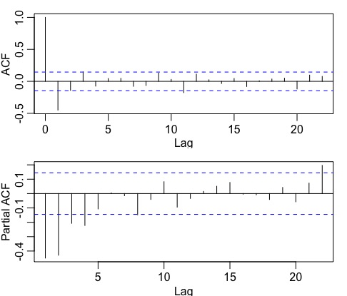
1. Supply the parameters p and q to the model. \(p = 2, q = 2\) in this case. Note that we pick p = 2 instead of p = 4 for a more parsimonious model.

2. Analyse residuals to make sure the fit is good and doesn’t violate any of the assumptions:

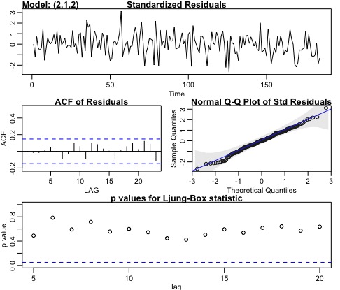
Analyzing our residuals,

• Normality assumption is met based on the Q-Q plot.
• Residuals look indepent identically distributed.
• As our p-value is greater than 0.5 in the Ljung–Box–Pierce Q-statistic it indicates that our ACF residuls follow a \(X^2\) distribution. Note that the null hypothesis, \(H_0\) here is that our residuals do not follow a chi-squared distribution.

But as we would like to forecast RUL for multiple engines, doing this for each engine is not effective. Therefore, we will use the auto.arima() function from the forecast package in R. This function returns the best ARIMA model according to either AIC, AICc or BIC value by conducting a search over possible model. Post that we create a custom function that will use auto.arima() to generate model order \(p,d,q\) and then forecast it’s RUL till it reaches 0.

#Our custom function uses the auto.arima() function from forecast package
#Forecasts till 10000 iterations or when our RUL reaches 0, whichever is earlier
RUL_list_arima = lapply(final_list2, function(x){
  out = auto.arima(x, d = 1, max.p = 15, max.q = 15)
  p = out$arma[1]
  q = out$arma[2]
  for(i in 1:10000){
    out_for = sarima.for(x, i, p,1,q)
    if (out_for$pred[i] <= 0.0){
      RUL = i
      break
    }
  }
  return(RUL)
})

Multilayer Perceptron (MLP)

A multilayer perceptron is a basic feed forward ANN network. In this post we implement MLP using the nnfor package in R. Neural networks are not great in modelling trends as in time series with trends the values are ever increasing/decreasing but the activation functions used within the network are bounded to \([0,1]\) or \([-1,1]\) depending on the activation funciton used i.e sigmoid and tanh respectively.

Therefore, in such cases with trends, differencing and scaling can help. However, there is a catch here. Note, that differencing will only be of use when we are dealing with a stochastic trend and absence of seasonality. If we have a series with trend and seasonality then by working on the differenced series we will be unable to approximate the underlying functional form of seasonality.

For this particular problem we will train a model on each of the 9 engines. We will be supplying lags of the series as inputs the default for the mlp() command is 3. We will have 5 hidden nodes in one single layer. The activation function used is sigmoid (by default). Additionally, we will also perform differencing, in alignment with the above KPSS test results, which is taken care by the model argument difforder.

Mathamatically, our model is:

\[\begin{aligned} \hat{y} = \beta_0 + \sum^5_{i=1}(w_i\sigma(\beta_{0,i}+\sum^3_{j=1}w_{j,i}X_j)) \end{aligned}\]

where \(\beta_0\) and \(\beta_{0,i}\) are the bias of the output and each node respectively. \(w_{j,i}\) and \(w_i\) are weights for each input \(X_j\) and hidden nodes \(H_i\).

We can clearly observe that each neuron is a conventional regression that passes through a sigmoid to become nonlinear. Inputs are passed via the nonlinear function multiple times and the results are combined in the output. This combination of several nonlinear approximations enables the neural network to map our series very well.

Training our model on the 9 engines

#Fitting a MLP to the 9 engines
RUL_list_mlp = lapply(forecast_list2, function(x){
  mlp_fit = mlp(x, difforder = 1) #passing the trained model as an argument
  for(i in 1:1000){
    out_for = forecast(mlp_fit, h = i)
    if (out_for$mean[i] <= 0.01){
      RUL = i
      break
    }
  }
  return(RUL)
})

Note that, the MLP function by default trains the model 20 times and the different forecasts are combined using the median operator.

Modelling this way is very very very computationally intensive and a workaround could be training one model on a series and then passing this model as an argument to forecast other models as well. This would use the weights and biases of the fitted model to forecast other time series. However, as we only have 9 engines we let the code run for now.

Analysis

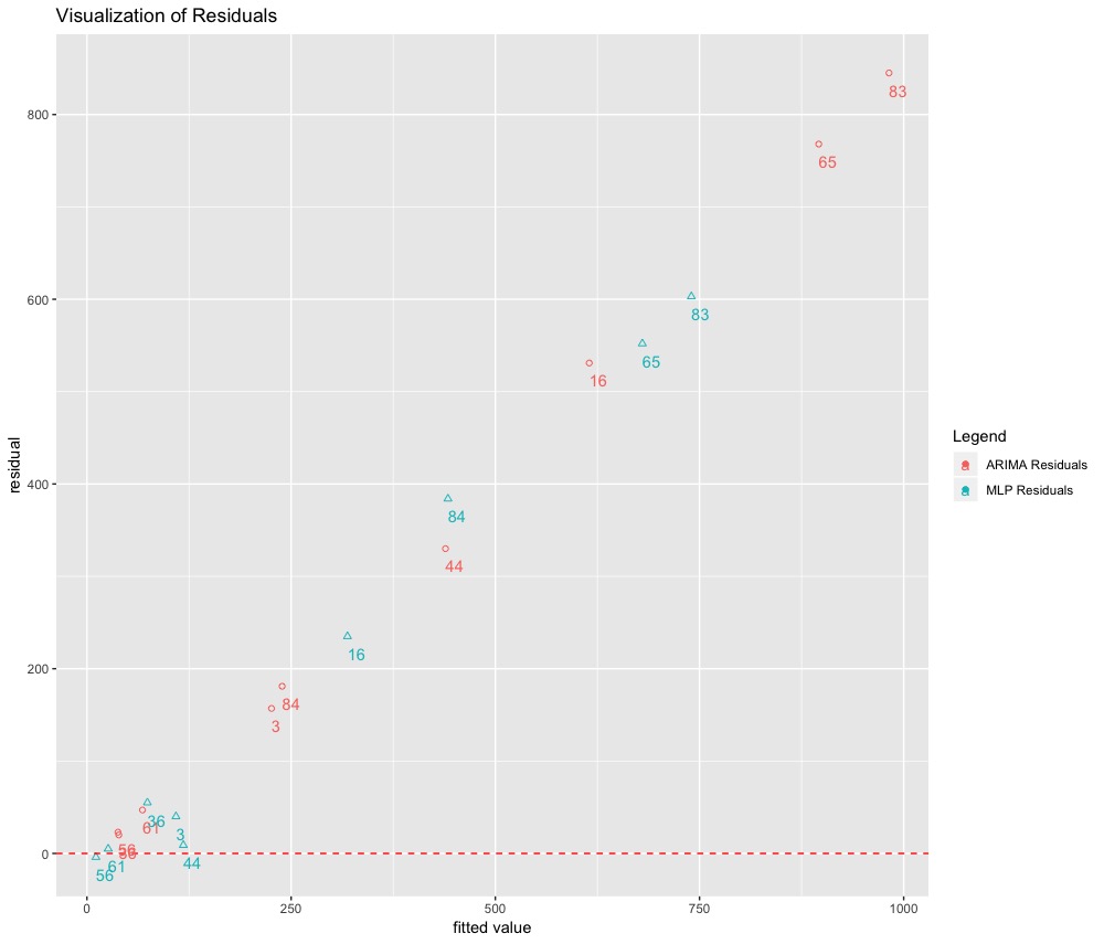
Now that we have our RUL predictions we will compute the residuals to visualize the results. Instead of using \(e = y - \hat{y}\) we will compute the residuals as \(e = \hat{y} - y\) where \(\hat{y}\) and \(y\) are the predicted and actual RUL respectively. We do this we would like to see how much we have over or under predicted. Below is a plot of our results:

ARIMA and MLP RUL predictions with Engine numbers

Here is a corresponding dataframe:

ARIMA and MLP forecasts and residuals along with RUL and Engine numbers

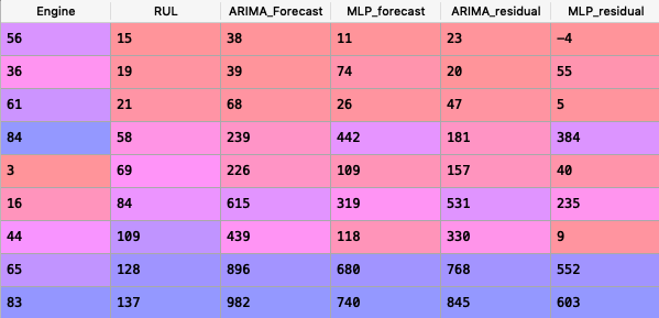
We can make 3 key observations:

• MLP prediction errors are much smaller than ARIMA’s for 7 of the 9 engines.
• There is a almost a linear trend in the errors of the ARIMA model. The errors get bigger as the RUL count increases. This means ARIMA performs poorly in estimating the life of our machine when many cyles are left.
• Introducing some non-linearity in our function has helped in forecating RUL.

However, this particular plot or the residuals we computed are not the best evaluation metric. The correct evaluation metric is mentioned in this paper associated with the PHM08 challenge.

The cost function provided is:

\[\begin{aligned} s = \begin{array}{ll} \sum_{n=1}^{n} e ^ {(-d/a_1)} - 1, d < 0 \\ \sum_{n=1}^{n} e ^ {(-d/a_2)} - 1, d \geq 0 \end{array} \end{aligned}\]

where:

• \(s\) is the computed score
• \(n\) is the number of UUT’s
• \(d\) = Estimated RUL - True RUL
• \(a_1\) = 10, \(a_2\) = 13

We can visualize the cost function using python:

#Plotting the cost function
x = np.arange(-50, 50, 1)
y = []
for i in x:
    if i<0:
        y.append(np.exp(-(i / 13)) - 1)
    else:
        y.append(np.exp(i/10) - 1)

plt.plot(x, y)
plt.ylabel('Score')
plt.xlabel('error')
plt.title('Plot of the Cost as a function of error')
plt.show()

This is how the asymmetric cost function looks:

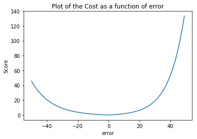
Note that the cost function is asymmetric as naturally for an engine degradation scenario an early prediction is preferred over late predictions. Therefore, the scoring algorithm for this challenge was asymmetric around the true time of failure such that late predictions were more heavily penalized than early predictions. As can be seen from the above equation the asymmetric preference is controlled by parameters \(a_1\) and \(a_2\).

Now let us apply this cost function to our values.

#Create a function to calculate the cost function
def cost_function(aplist):
    d = aplist[1] - aplist[0] #Estimated - True
    if d<0:
        s = math.exp(-(d/13)) - 1
    else:
        s = math.exp(d/10)-1
    return(s)


#First, for the ARIMA case
arima_cost = forecast_df[['RUL', 'ARIMA_Forecast']]
arima_cost = arima_cost.values
arima_cost = arima_cost.tolist()

arima_value = []
for i in arima_cost:
    arima_value.append(cost_function(i))


#Second, for the MLP case
mlp_cost = forecast_df[['RUL', 'MLP_forecast']]
mlp_cost = mlp_cost.values
mlp_cost = mlp_cost.tolist()

mlp_value = []
for i in mlp_cost:
    mlp_value.append(cost_function(i))

#create a final scores df
score_df = pd.DataFrame({'ARIMA_score': arima_value,
              'MLP_score': mlp_value})
final_score_df = pd.concat([forecast_df[['Engine', 'RUL']], score_df], axis=1)
final_score_df.to_csv('final_score_df.csv', index = False)

Below is a screenshot of our results:

Score of our models on the 9 Engines.

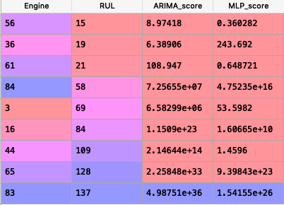
We can observe that MLP beats ARIMA on all the engines except 36 and 84 where it gave a forecast of 55 in comparision to ARIMA’s 20 and 384 in comparision to 181.

Conclusion

Based on our analysis we can conclude that using nonlinearity to map our univariate series can give us better perfomance in forecasting RUL. However, the MLP approach used here is quite difficult to train as the values don’t necessarily converge to 0 everytime. We observe, that the ARIMA is devoid of this problem and always converges to 0. However, it is not practical to use ARIMA while forecasting machines with large RUL.

References

Saxena, A., Goebel, K., Simon, D., & Eklund, N. (2008). Damage propagation modeling for aircraft engine run-to-failure simulation. 2008 International Conference on Prognostics and Health Management. doi:10.1109/phm.2008.4711414

Elattar, H. (n.d.). Intelligent information system to forecast the remaining life of aircraft turbofan engine.

Riad, A. (n.d.). Evaluation of Neural Networks in the Subject of Prognostics As Compared To Linear Regression Model.

Zhao, J., Xu, L., & Liu, L. (2007). Equipment Fault Forecasting Based on ARMA Model. 2007 International Conference on Mechatronics and Automation. doi:10.1109/icma.2007.4304129

Code for this article can be found here.